


Introduction
Treat "forests" well. Not for the sake of nature, but for solving problems too!
Random Forest is one of the most versatile machine learning algorithms available today. With its built-in ensembling capacity, the task of building a decent generalized model (on any dataset) gets much easier. However, I've seen people using random forest as a black box model; i.e., they don't understand what's happening beneath the code. They just code.
In fact, the easiest part of machine learning is coding. If you are new to machine learning, the random forest algorithm should be on your tips. Its ability to solve—both regression and classification problems along with robustness to correlated features and variable importance plot gives us enough head start to solve various problems.
Most often, I've seen people getting confused in bagging and random forest. Do you know the difference?
In this article, I'll explain the complete concept of random forest and bagging. For ease of understanding, I've kept the explanation simple yet enriching. I've used MLR, data.table packages to implement bagging, and random forest with parameter tuning in R. Also, you'll learn the techniques I've used to improve model accuracy from ~82% to 86%.
Table of Contents
- What is the Random Forest algorithm?
- How does it work? (Decision Tree, Random Forest)
- What is the difference between Bagging and Random Forest?
- Advantages and Disadvantages of Random Forest
- Solving a Problem
- Parameter Tuning in Random Forest
What is the Random Forest algorithm?
Random forest is a tree-based algorithm which involves building several trees (decision trees), then combining their output to improve generalization ability of the model. The method of combining trees is known as an ensemble method. Ensembling is nothing but a combination of weak learners (individual trees) to produce a strong learner.
Say, you want to watch a movie. But you are uncertain of its reviews. You ask 10 people who have watched the movie. 8 of them said "the movie is fantastic." Since the majority is in favor, you decide to watch the movie. This is how we use ensemble techniques in our daily life too.
Random Forest can be used to solve regression and classification problems. In regression problems, the dependent variable is continuous. In classification problems, the dependent variable is categorical.
Trivia: The random Forest algorithm was created by Leo Breiman and Adele Cutler in 2001.
How does it work? (Decision Tree, Random Forest)
To understand the working of a random forest, it's crucial that you understand a tree. A tree works in the following way:
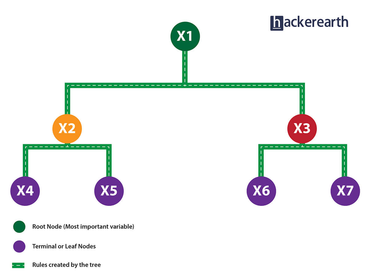
1. Given a data frame (n x p), a tree stratifies or partitions the data based on rules (if-else). Yes, a tree creates rules. These rules divide the data set into distinct and non-overlapping regions. These rules are determined by a variable's contribution to the homogeneity or pureness of the resultant child nodes (X2, X3).
2. In the image above, the variable X1 resulted in highest homogeneity in child nodes, hence it became the root node. A variable at root node is also seen as the most important variable in the data set.
3. But how is this homogeneity or pureness determined? In other words, how does the tree decide at which variable to split?
- In regression trees (where the output is predicted using the mean of observations in the terminal nodes), the splitting decision is based on minimizing RSS. The variable which leads to the greatest possible reduction in RSS is chosen as the root node. The tree splitting takes a top-down greedy approach, also known as recursive binary splitting. We call it "greedy" because the algorithm cares to make the best split at the current step rather than saving a split for better results on future nodes.
- In classification trees (where the output is predicted using mode of observations in the terminal nodes), the splitting decision is based on the following methods:
- Gini Index - It's a measure of node purity. If the Gini index takes on a smaller value, it suggests that the node is pure. For a split to take place, the Gini index for a child node should be less than that for the parent node.
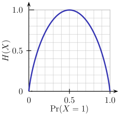
- Entropy - Entropy is a measure of node impurity. For a binary class (a, b), the formula to calculate it is shown below. Entropy is maximum at p = 0.5. For p(X=a)=0.5 or p(X=b)=0.5 means a new observation has a 50%-50% chance of getting classified in either class. The entropy is minimum when the probability is 0 or 1.
Entropy = - p(a)*log(p(a)) - p(b)*log(p(b))
In a nutshell, every tree attempts to create rules in such a way that the resultant terminal nodes could be as pure as possible. Higher the purity, lesser the uncertainty to make the decision.
But a decision tree suffers from high variance. "High Variance" means getting high prediction error on unseen data. We can overcome the variance problem by using more data for training. But since the data set available is limited to us, we can use resampling techniques like bagging and random forest to generate more data.
Building many decision trees results in a forest. A random forest works the following way:
- First, it uses the Bagging (Bootstrap Aggregating) algorithm to create random samples. Given a data set D1 (n rows and p columns), it creates a new dataset (D2) by sampling n cases at random with replacement from the original data. About 1/3 of the rows from D1 are left out, known as Out of Bag (OOB) samples.
- Then, the model trains on D2. OOB sample is used to determine unbiased estimate of the error.
- Out of p columns, P ≪ p columns are selected at each node in the data set. The P columns are selected at random. Usually, the default choice of P is p/3 for regression tree and √p for classification tree.
-
 Unlike a tree, no pruning takes place in random forest; i.e., each tree is grown fully. In decision trees, pruning is a method to avoid overfitting. Pruning means selecting a subtree that leads to the lowest test error rate. We can use cross-validation to determine the test error rate of a subtree.
- Several trees are grown and the final prediction is obtained by averaging (for regression) or majority voting (for classification).
Each tree is grown on a different sample of original data. Since random forest has the feature to calculate OOB error internally, cross-validation doesn't make much sense in random forest.
What is the difference between Bagging and Random Forest?
Many a time, we fail to ascertain that bagging is not the same as random forest. To understand the difference, let's see how bagging works:
- It creates randomized samples of the dataset (just like random forest) and grows trees on a different sample of the original data. The remaining 1/3 of the sample is used to estimate unbiased OOB error.
- It considers all the features at a node (for splitting).
- Once the trees are fully grown, it uses averaging or voting to combine the resultant predictions.
Aren't you thinking, "If both the algorithms do the same thing, what is the need for random forest? Couldn't we have accomplished our task with bagging?" NO!
The need for random forest surfaced after discovering that the bagging algorithm results in correlated trees when faced with a dataset having strong predictors. Unfortunately, averaging several highly correlated trees doesn't lead to a large reduction in variance.
But how do correlated trees emerge? Good question! Let's say a dataset has a very strong predictor, along with other moderately strong predictors. In bagging, a tree grown every time would consider the very strong predictor at its root node, thereby resulting in trees similar to each other.
The main difference between random forest and bagging is that random forest considers only a subset of predictors at a split. This results in trees with different predictors at the top split, thereby resulting in decorrelated trees and more reliable average output. That's why we say random forest is robust to correlated predictors.
Advantages and Disadvantages of Random Forest
Advantages are as follows:
- It is robust to correlated predictors.
- It is used to solve both regression and classification problems.
- It can also be used to solve unsupervised ML problems.
- It can handle thousands of input variables without variable selection.
- It can be used as a feature selection tool using its variable importance plot.
- It takes care of missing data internally in an effective manner.
Disadvantages are as follows:
- The Random Forest model is difficult to interpret.
- It tends to return erratic predictions for observations out of the range of training data. For example, if the training data contains a variable x ranging from 30 to 70, and the test data has x = 200, random forest would give an unreliable prediction.
- It can take longer than expected to compute a large number of trees.
Solving a Problem (Parameter Tuning)
Let's take a dataset to compare the performance of bagging and random forest algorithms. Along the way, I'll also explain important parameters used for parameter tuning. In R, we'll use MLR and data.table packages to do this analysis.
I've taken the Adult dataset from the UCI machine learning repository. You can download the data from here.
This dataset presents a binary classification problem to solve. Given a set of features, we need to predict if a person's salary is <=50K or >=50K. Since the given data isn't well structured, we'll need to make some modification while reading the dataset.
# set working directory
path <- "~/December 2016/RF_Tutorial"
setwd(path)
# Set working directory
path <- "~/December 2016/RF_Tutorial"
setwd(path)

# Load libraries
library(data.table)
library(mlr)
library(h2o)

# Set variable names
setcol <- c("age",
            "workclass",
            "fnlwgt",
            "education",
            "education-num",
            "marital-status",
            "occupation",
            "relationship",
            "race",
            "sex",
            "capital-gain",
            "capital-loss",
            "hours-per-week",
            "native-country",
            "target")

# Load data
train <- read.table("adultdata.txt", header = FALSE, sep = ",",
                    col.names = setcol, na.strings = c(" ?"), stringsAsFactors = FALSE)
test <- read.table("adulttest.txt", header = FALSE, sep = ",",
                   col.names = setcol, skip = 1, na.strings = c(" ?"), stringsAsFactors = FALSE)
After we've loaded the dataset, first we'll set the data class to data.table. data.table is the most powerful R package made for faster data manipulation.
>setDT(train)
>setDT(test)
Now, we'll quickly look at given variables, data dimensions, etc.
>dim(train)
>dim(test)
>str(train)
>str(test)
As seen from the output above, we can derive the following insights:
- The train dataset has 32,561 rows and 15 columns.
- The test dataset has 16,281 rows and 15 columns.
- Variable
targetis the dependent variable. - The target variable in train and test data is different. We'll need to match them.
- All character variables have a leading whitespace which can be removed.
We can check missing values using:
# Check missing values in train and test datasets
>table(is.na(train))
# Output:
#  FALSE   TRUE
#  484153  4262

>sapply(train, function(x) sum(is.na(x)) / length(x)) * 100

table(is.na(test))
# Output:
#  FALSE  TRUE
#  242012 2203

>sapply(test, function(x) sum(is.na(x)) / length(x)) * 100
As seen above, both train and test datasets have missing values. The sapply function is quite handy when it comes to performing column computations. Above, it returns the percentage of missing values per column.
Now, we'll preprocess the data to prepare it for training. In R, random forest internally takes care of missing values using mean/mode imputation. Practically speaking, sometimes it takes longer than expected for the model to run.
Therefore, in order to avoid waiting time, let's impute the missing values using median/mode imputation method; i.e., missing values in the integer variables will be imputed with median and in the factor variables with mode (most frequent value).
We'll use the impute function from the mlr package, which is enabled with several unique methods for missing value imputation:
# Impute missing values
>imp1 <- impute(data = train, target = "target",
              classes = list(integer = imputeMedian(), factor = imputeMode()))

>imp2 <- impute(data = test, target = "target",
              classes = list(integer = imputeMedian(), factor = imputeMode()))

# Assign the imputed data back to train and test
>train <- imp1$data
>test <- imp2$data
Being a binary classification problem, you are always advised to check if the data is imbalanced or not. We can do it in the following way:
# Check class distribution in train and test datasets
setDT(train)[, .N / nrow(train), target]
# Output:
#    target     V1
# 1: <=50K   0.7591904
# 2: >50K    0.2408096

setDT(test)[, .N / nrow(test), target]
# Output:
#    target     V1
# 1: <=50K.  0.7637737
# 2: >50K.   0.2362263
If you observe carefully, the value of the target variable is different in test and train. For now, we can consider it a typo error and correct all the test values. Also, we see that 75% of people in the train data have income <=50K. Imbalanced classification problems are known to be more skewed with a binary class distribution of 90% to 10%. Now, let's proceed and clean the target column in test data.
# Clean trailing character in test target values
test[, target := substr(target, start = 1, stop = nchar(target) - 1)]
We've used the substr function to return the substring from a specified start and end position. Next, we'll remove the leading whitespaces from all character variables. We'll use the str_trim function from the stringr package.
> library(stringr)
> char_col <- colnames(train)[sapply(train, is.character)]
> for(i in char_col)
>     set(train, j = i, value = str_trim(train[[i]], side = "left"))
Using sapply function, we've extracted the column names which have character class. Then, using a simple for - set loop we traversed all those columns and applied the str_trim function.
Before we start model training, we should convert all character variables to factor. MLR package treats character class as unknown.
> fact_col <- colnames(train)[sapply(train,is.character)]
>for(i in fact_col)
			set(train,j=i,value = factor(train[[i]]))
>for(i in fact_col)
	     set(test,j=i,value = factor(test[[i]]))
Let's start with modeling now. MLR package has its own function to convert data into a task, build learners, and optimize learning algorithms. I suggest you stick to the modeling structure described below for using MLR on any data set.
#create a task
> traintask <- makeClassifTask(data = train,target = "target")
> testtask <- makeClassifTask(data = test,target = "target")

#create learner
> bag <- makeLearner("classif.rpart",predict.type = "response")
> bag.lrn <- makeBaggingWrapper(learner = bag,bw.iters = 100,bw.replace = TRUE)
I've set up the bagging algorithm which will grow 100 trees on randomized samples of data with replacement. To check the performance, let's set up a validation strategy too:
#set 5 fold cross validation
> rdesc <- makeResampleDesc("CV", iters = 5L)
For faster computation, we'll use parallel computation backend. Make sure your machine / laptop doesn't have many programs running in the background.
#set parallel backend (Windows)
> library(parallelMap)
> library(parallel)
> parallelStartSocket(cpus = detectCores())
For linux users, the function parallelStartMulticore(cpus = detectCores()) will activate parallel backend. I've used all the cores here.
r <- resample(learner = bag.lrn,
              task = traintask,
              resampling = rdesc,
              measures = list(tpr, fpr, fnr, fpr, acc),
              show.info = T)

#[Resample] Result:
# tpr.test.mean = 0.95,
# fnr.test.mean = 0.0505,
# fpr.test.mean = 0.487,
# acc.test.mean = 0.845
Being a binary classification problem, I've used the components of confusion matrix to check the model's accuracy. With 100 trees, bagging has returned an accuracy of 84.5%, which is way better than the baseline accuracy of 75%. Let's now check the performance of random forest.
#make randomForest learner
> rf.lrn <- makeLearner("classif.randomForest")
> rf.lrn$par.vals <- list(ntree = 100L,
                          importance = TRUE)

> r <- resample(learner = rf.lrn,
                task = traintask,
                resampling = rdesc,
                measures = list(tpr, fpr, fnr, fpr, acc),
                show.info = T)

# Result:
# tpr.test.mean = 0.996,
# fpr.test.mean = 0.72,
# fnr.test.mean = 0.0034,
# acc.test.mean = 0.825
On this data set, random forest performs worse than bagging. Both used 100 trees and random forest returns an overall accuracy of 82.5 %. An apparent reason being that this algorithm is messing up classifying the negative class. As you can see, it classified 99.6% of the positive classes correctly, which is way better than the bagging algorithm. But it incorrectly classified 72% of the negative classes.
Internally, random forest uses a cutoff of 0.5; i.e., if a particular unseen observation has a probability higher than 0.5, it will be classified as <=50K. In random forest, we have the option to customize the internal cutoff. As the false positive rate is very high now, we'll increase the cutoff for positive classes (<=50K) and accordingly reduce it for negative classes (>=50K). Then, train the model again.
#set cutoff
> rf.lrn$par.vals <- list(ntree = 100L,
                          importance = TRUE,
                          cutoff = c(0.75, 0.25))

> r <- resample(learner = rf.lrn,
                task = traintask,
                resampling = rdesc,
                measures = list(tpr, fpr, fnr, fpr, acc),
                show.info = T)

#Result:
# tpr.test.mean = 0.934,
# fpr.test.mean = 0.43,
# fnr.test.mean = 0.0662,
# acc.test.mean = 0.846
As you can see, we've improved the accuracy of the random forest model by 2%, which is slightly higher than that for the bagging model. Now, let's try and make this model better.
Parameter Tuning: Mainly, there are three parameters in the random forest algorithm which you should look at (for tuning):
- ntree - As the name suggests, the number of trees to grow. Larger the tree, it will be more computationally expensive to build models.
- mtry - It refers to how many variables we should select at a node split. Also as mentioned above, the default value is p/3 for regression and sqrt(p) for classification. We should always try to avoid using smaller values of mtry to avoid overfitting.
- nodesize - It refers to how many observations we want in the terminal nodes. This parameter is directly related to tree depth. Higher the number, lower the tree depth. With lower tree depth, the tree might even fail to recognize useful signals from the data.
Let get to the playground and try to improve our model's accuracy further. In MLR package, you can list all tuning parameters a model can support using:
> getParamSet(rf.lrn)

# set parameter space
params <- makeParamSet(
    makeIntegerParam("mtry", lower = 2, upper = 10),
    makeIntegerParam("nodesize", lower = 10, upper = 50)
)

# set validation strategy
rdesc <- makeResampleDesc("CV", iters = 5L)

# set optimization technique
ctrl <- makeTuneControlRandom(maxit = 5L)

# start tuning
> tune <- tuneParams(learner = rf.lrn,
                     task = traintask,
                     resampling = rdesc,
                     measures = list(acc),
                     par.set = params,
                     control = ctrl,
                     show.info = T)

[Tune] Result: mtry=2; nodesize=23 : acc.test.mean=0.858
After tuning, we have achieved an overall accuracy of 85.8%, which is better than our previous random forest model. This way you can tweak your model and improve its accuracy.
I'll leave you here. The complete code for this analysis can be downloaded from Github.
Summary
Don't stop here! There is still a huge scope for improvement in this model. Cross validation accuracy is generally more optimistic than true test accuracy. To make a prediction on the test set, minimal data preprocessing on categorical variables is required. Do it and share your results in the comments below.
My motive to create this tutorial is to get you started using the random forest model and some techniques to improve model accuracy. For better understanding, I suggest you read more on confusion matrix. In this article, I've explained the working of decision trees, random forest, and bagging.
Did I miss out anything? Do share your knowledge and let me know your experience while solving classification problems in comments below.


