


from the UC Irivine ML repository. Let's start with H2O. This data set isn't the most ideal one to work with in neural networks. However, the motive of this hands-on section is to make you familiar with model-building processes.
Now, let's build a simple deep learning model. Generally, computing variable importance from a trained deep learning model is quite pain staking. But, h2o package provides an effortless function to compute variable importance from a deep learning model.

Now, let's train a deep learning model with one hidden layer comprising five neurons. This time instead of checking the cross-validation accuracy, we'll validate the model on test data.
For hyperparameter tuning, we'll perform a random grid search over all parameters and choose the model which returns highest accuracy.
In R, mxnet accepts target variables as numeric classes and not factors. Also, it accepts data frame as a matrix. Now, we'll make the required changes:
Now, we'll train the multilayered perceptron model using the mx.mlp function.
Softmax function is used for binary and multi-classification problems. Alternatively, you can also manually craft the model structure.
We have configured the network above with one hidden layer carrying three neurons. We have chosen softmax as the output function. The network optimizes for squared loss for regression, and the network optimizes for classification accuracy for classification. Now, we'll train the network:
Similarly, we can configure a more complexed network fed with hidden layers.
Understand it carefully: After feeding the input through data, the first hidden layer consists of 10 neurons. The output of each neuron passes through a relu (rectified linear) activation function. We have used it in place of sigmoid. relu converges faster than a sigmoid function. You can read more about relu here.
Then, the output is fed into the second layer which is the output layer. Since our target variable has two classes, we've chosen num_hidden as 2 in the second layer. Finally, the output from second layer is made to pass though softmax output function.
As mentioned above, this trained model predicts output probability, which can be easily transformed into a label using a threshold value (say, 0.5). To make predictions on the test set, we do this:
The predicted matrix returns two rows and 16281 columns, each column carrying probability. Using the max.col function, we can extract the maximum value from each row. If you check the model's accuracy, you'll find that this network performs terribly on this data. In fact, it gives no better result than the train accuracy! On this data set, xgboost tuning gave 87% accuracy!
If you are familiar with the model building process, I'd suggest you to try working on the popular MNIST data set. You can find tons of tutorials on this data to get you going!
H2O Package
H2O package providesh2o.deeplearning function for model building. It is built on Java. Primarily, this function is useful to build multilayer feedforward neural networks. It is enabled with several features such as the following:- Multi-threaded distributed parallel computation
- Adaptive learning rate (or step size) for faster convergence
- Regularization options such as L1 and L2 which help prevent overfitting
- Automatic missing value imputation
- Hyperparameter optimization using grid/random search
- hidden - It specifies the number of hidden layers and number of neurons in each layer in the architechture.
- epochs - It specifies the number of iterations to be done on the data set.
- rate - It specifies the learning rate.
- activation - It specifies the type of activation function to use. In h2o, the major activation functions are Tanh, Rectifier, and Maxout.
This file contains hidden or bidirectional Unicode text that may be interpreted or compiled differently than what appears below. To review, open the file in an editor that reveals hidden Unicode characters.
Learn more about bidirectional Unicode characters
| path = "~/mydata/deeplearning" | |
| setwd(path) | |
| #load libraries | |
| library(data.table) | |
| library(mlr) | |
| #set variable names | |
| setcol <- c("age", | |
| "workclass", | |
| "fnlwgt", | |
| "education", | |
| "education-num", | |
| "marital-status", | |
| "occupation", | |
| "relationship", | |
| "race", | |
| "sex", | |
| "capital-gain", | |
| "capital-loss", | |
| "hours-per-week", | |
| "native-country", | |
| "target") | |
| #load data | |
| train <- read.table("adultdata.txt",header = F,sep = ",",col.names = setcol,na.strings = c(" ?"),stringsAsFactors = F) | |
| test <- read.table("adulttest.txt",header = F,sep = ",",col.names = setcol,skip = 1, na.strings = c(" ?"),stringsAsFactors = F) | |
| setDT(train) | |
| setDT(test) | |
| #Data Sanity | |
| dim(train) #32561 X 15 | |
| dim(test) #16281 X 15 | |
| str(train) | |
| str(test) | |
| #check missing values | |
| table(is.na(train)) | |
| sapply(train, function(x) sum(is.na(x))/length(x))*100 | |
| table(is.na(test)) | |
| sapply(test, function(x) sum(is.na(x))/length(x))*100 | |
| #check target variable | |
| #binary in nature check if data is imbalanced | |
| train[,.N/nrow(train),target] | |
| test[,.N/nrow(test),target] | |
| #remove extra characters | |
| test[,target := substr(target,start = 1,stop = nchar(target)-1)] | |
| #remove leading whitespace | |
| library(stringr) | |
| char_col <- colnames(train)[sapply(test,is.character)] | |
| for(i in char_col) | |
| set(train,j=i,value = str_trim(train[[i]],side = "left")) | |
| #set all character variables as factor | |
| fact_col <- colnames(train)[sapply(train,is.character)] | |
| for(i in fact_col) | |
| set(train,j=i,value = factor(train[[i]])) | |
| for(i in fact_col) | |
| set(test,j=i,value = factor(test[[i]])) | |
| #impute missing values | |
| imp1 <- impute(data = train,target = "target",classes = list(integer = imputeMedian(), factor = imputeMode())) | |
| imp2 <- impute(data = test,target = "target",classes = list(integer = imputeMedian(), factor = imputeMode())) | |
| train <- setDT(imp1$data) | |
| test <- setDT(imp2$data) |
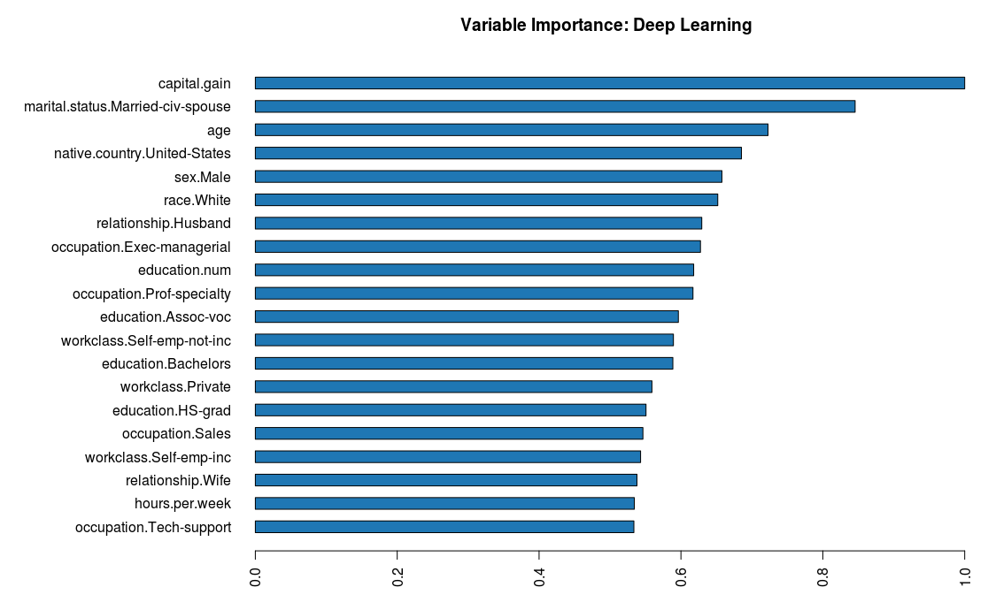
Now, let's build a simple deep learning model. Generally, computing variable importance from a trained deep learning model is quite pain staking. But, h2o package provides an effortless function to compute variable importance from a deep learning model.
This file contains hidden or bidirectional Unicode text that may be interpreted or compiled differently than what appears below. To review, open the file in an editor that reveals hidden Unicode characters.
Learn more about bidirectional Unicode characters
| #load the package | |
| require(h2o) | |
| #start h2o | |
| localH2o <- h2o.init(nthreads = -1, max_mem_size = "20G") | |
| #load data on H2o | |
| trainh2o <- as.h2o(train) | |
| testh2o <- as.h2o(test) | |
| #set variables | |
| y <- "target" | |
| x <- setdiff(colnames(trainh2o),y) | |
| #train the model - without hidden layer | |
| deepmodel <- h2o.deeplearning(x = x | |
| ,y = y | |
| ,training_frame = trainh2o | |
| ,standardize = T | |
| ,model_id = "deep_model" | |
| ,activation = "Rectifier" | |
| ,epochs = 100 | |
| ,seed = 1 | |
| ,nfolds = 5 | |
| ,variable_importances = T) | |
| #compute variable importance and performance | |
| h2o.varimp_plot(deepmodel,num_of_features = 20) | |
| h2o.performance(deepmodel,xval = T) #84.5 % CV accuracy |
Now, let's train a deep learning model with one hidden layer comprising five neurons. This time instead of checking the cross-validation accuracy, we'll validate the model on test data.
This file contains hidden or bidirectional Unicode text that may be interpreted or compiled differently than what appears below. To review, open the file in an editor that reveals hidden Unicode characters.
Learn more about bidirectional Unicode characters
| deepmodel <- h2o.deeplearning(x = x | |
| ,y = y | |
| ,training_frame = trainh2o | |
| ,validation_frame = testh2o | |
| ,standardize = T | |
| ,model_id = "deep_model" | |
| ,activation = "Rectifier" | |
| ,epochs = 100 | |
| ,seed = 1 | |
| ,hidden = 5 | |
| ,variable_importances = T) | |
| h2o.performance(deepmodel,valid = T) #85.6% |
For hyperparameter tuning, we'll perform a random grid search over all parameters and choose the model which returns highest accuracy.
This file contains hidden or bidirectional Unicode text that may be interpreted or compiled differently than what appears below. To review, open the file in an editor that reveals hidden Unicode characters.
Learn more about bidirectional Unicode characters
| #set parameter space | |
| activation_opt <- c("Rectifier","RectifierWithDropout", "Maxout","MaxoutWithDropout") | |
| hidden_opt <- list(c(10,10),c(20,15),c(50,50,50)) | |
| l1_opt <- c(0,1e-3,1e-5) | |
| l2_opt <- c(0,1e-3,1e-5) | |
| hyper_params <- list( activation=activation_opt, | |
| hidden=hidden_opt, | |
| l1=l1_opt, | |
| l2=l2_opt ) | |
| #set search criteria | |
| search_criteria <- list(strategy = "RandomDiscrete", max_models=10) | |
| #train model | |
| dl_grid <- h2o.grid("deeplearning" | |
| ,grid_id = "deep_learn" | |
| ,hyper_params = hyper_params | |
| ,search_criteria = search_criteria | |
| ,training_frame = trainh2o | |
| ,x=x | |
| ,y=y | |
| ,nfolds = 5 | |
| ,epochs = 100) | |
| #get best model | |
| d_grid <- h2o.getGrid("deep_learn",sort_by = "accuracy") | |
| best_dl_model <- h2o.getModel(d_grid@model_ids[[1]]) | |
| h2o.performance (best_dl_model,xval = T) #CV Accuracy - 84.7% |
MXNetR Package
The mxnet package provides an incredible interface to build feedforward NN, recurrent NN and convolutional neural networks (CNNs). CNNs are being widely used in detecting objects from images. The team that created xgboost also created this package. Currently, mxnet is being popularly used in kaggle competitions for image classification problems.This package can be easily connected with GPUs as well. The process of building model architecture is quite intuitive. It gives greater control to configure the neural network manually.
Let's get some hands-on experience using this package.Follow the commands below to install this package in your respective OS. For Windows and Linux users, installation commands are given below. For Mac users, here's the installation procedure.
This file contains hidden or bidirectional Unicode text that may be interpreted or compiled differently than what appears below. To review, open the file in an editor that reveals hidden Unicode characters.
Learn more about bidirectional Unicode characters
| # # Installation - Windows | |
| install.packages("drat", repos="https://cran.rstudio.com") | |
| drat:::addRepo("dmlc") | |
| install.packages("mxnet") | |
| library(mxnet) | |
| #Installation - Linux | |
| #Press Ctrl + Alt + T and run the following command | |
| sudo apt-get update | |
| sudo apt-get -y install git | |
| git clone https://github.com/dmlc/mxnet.git ~/mxnet --recursive | |
| cd ~/mxnet/setup-utils | |
| bash install-mxnet-ubuntu-r.sh |
In R, mxnet accepts target variables as numeric classes and not factors. Also, it accepts data frame as a matrix. Now, we'll make the required changes:
This file contains hidden or bidirectional Unicode text that may be interpreted or compiled differently than what appears below. To review, open the file in an editor that reveals hidden Unicode characters.
Learn more about bidirectional Unicode characters
| #load package | |
| require(mxnet) | |
| #convert target variables into numeric | |
| train[,target := as.numeric(target)-1] | |
| test[,target := as.numeric(target)-1] | |
| #convert train data to matrix | |
| train.x <- data.matrix(train[,-c("target"),with=F]) | |
| train.y <- train$target | |
| #convert test data to matrix | |
| test.x <- data.matrix(test[,-c("target"),with=F]) | |
| test.y <- test$target |
Now, we'll train the multilayered perceptron model using the mx.mlp function.
This file contains hidden or bidirectional Unicode text that may be interpreted or compiled differently than what appears below. To review, open the file in an editor that reveals hidden Unicode characters.
Learn more about bidirectional Unicode characters
| #set seed to reproduce results | |
| mx.set.seed(1) | |
| mlpmodel <- mx.mlp(data = train.x | |
| ,label = train.y | |
| ,hidden_node = 3 #one layer with 10 nodes | |
| ,out_node = 2 | |
| ,out_activation = "softmax" #softmax return probability | |
| ,num.round = 100 #number of iterations over training data | |
| ,array.batch.size = 20 #after every batch weights will get updated | |
| ,learning.rate = 0.03 #same as step size | |
| ,eval.metric= mx.metric.accuracy | |
| ,eval.data = list(data = test.x, label = test.y)) |
Softmax function is used for binary and multi-classification problems. Alternatively, you can also manually craft the model structure.
This file contains hidden or bidirectional Unicode text that may be interpreted or compiled differently than what appears below. To review, open the file in an editor that reveals hidden Unicode characters.
Learn more about bidirectional Unicode characters
| #create NN structure | |
| data <- mx.symbol.Variable("data") | |
| fc1 <- mx.symbol.FullyConnected(data, num_hidden=3) #3 neuron in one layer | |
| lrm <- mx.symbol.SoftmaxOutput(fc1) |
We have configured the network above with one hidden layer carrying three neurons. We have chosen softmax as the output function. The network optimizes for squared loss for regression, and the network optimizes for classification accuracy for classification. Now, we'll train the network:
This file contains hidden or bidirectional Unicode text that may be interpreted or compiled differently than what appears below. To review, open the file in an editor that reveals hidden Unicode characters.
Learn more about bidirectional Unicode characters
| nnmodel <- mx.model.FeedForward.create(symbol = lrm | |
| ,X = train.x | |
| ,y = train.y | |
| ,ctx = mx.cpu() | |
| ,num.round = 100 | |
| ,eval.metric = mx.metric.accuracy | |
| ,array.batch.size = 50 | |
| ,learning.rate = 0.01) |
Similarly, we can configure a more complexed network fed with hidden layers.
This file contains hidden or bidirectional Unicode text that may be interpreted or compiled differently than what appears below. To review, open the file in an editor that reveals hidden Unicode characters.
Learn more about bidirectional Unicode characters
| #configure another network | |
| data <- mx.symbol.Variable("data") | |
| fc1 <- mx.symbol.FullyConnected(data, name = "fc1", num_hidden=10) #1st hidden layer | |
| act1 <- mx.symbol.Activation(fc1, name = "sig", act_type="relu") | |
| fc2 <- mx.symbol.FullyConnected(act1, name = "fc2", num_hidden=2) #2nd hidden layer | |
| out <- mx.symbol.SoftmaxOutput(fc2, name = "soft") |
Understand it carefully: After feeding the input through data, the first hidden layer consists of 10 neurons. The output of each neuron passes through a relu (rectified linear) activation function. We have used it in place of sigmoid. relu converges faster than a sigmoid function. You can read more about relu here.
Then, the output is fed into the second layer which is the output layer. Since our target variable has two classes, we've chosen num_hidden as 2 in the second layer. Finally, the output from second layer is made to pass though softmax output function.
This file contains hidden or bidirectional Unicode text that may be interpreted or compiled differently than what appears below. To review, open the file in an editor that reveals hidden Unicode characters.
Learn more about bidirectional Unicode characters
| #train the network | |
| dp_model <- mx.model.FeedForward.create(symbol = out | |
| ,X = train.x | |
| ,y = train.y | |
| ,ctx = mx.cpu() | |
| ,num.round = 100 | |
| ,eval.metric = mx.metric.accuracy | |
| ,array.batch.size = 50 | |
| ,learning.rate = 0.005) |
As mentioned above, this trained model predicts output probability, which can be easily transformed into a label using a threshold value (say, 0.5). To make predictions on the test set, we do this:
This file contains hidden or bidirectional Unicode text that may be interpreted or compiled differently than what appears below. To review, open the file in an editor that reveals hidden Unicode characters.
Learn more about bidirectional Unicode characters
| #predict on test | |
| pred_dp <- predict(dp_model,test.x) | |
| str(pred_dp) #contains 2 rows and 16281 columns | |
| #transpose the pred matrix | |
| pred.val <- max.col(t(pred_dp))-1 |
The predicted matrix returns two rows and 16281 columns, each column carrying probability. Using the max.col function, we can extract the maximum value from each row. If you check the model's accuracy, you'll find that this network performs terribly on this data. In fact, it gives no better result than the train accuracy! On this data set, xgboost tuning gave 87% accuracy!
If you are familiar with the model building process, I'd suggest you to try working on the popular MNIST data set. You can find tons of tutorials on this data to get you going!


