Home
/
Blog
/
Developer Insights
/
Practical Tutorial on Random Forest and Parameter Tuning in R

Practical Tutorial on Random Forest and Parameter Tuning in R

Author
Manish Saraswat
Calendar Icon
December 14, 2016
Timer Icon
15 min read
Share

Introduction

Treat "forests" well. Not for the sake of nature, but for solving problems too!

Random Forest is one of the most versatile machine learning algorithms available today. With its built-in ensembling capacity, the task of building a decent generalized model (on any dataset) gets much easier. However, I've seen people using random forest as a black box model; i.e., they don't understand what's happening beneath the code. They just code.

In fact, the easiest part of machine learning is coding. If you are new to machine learning, the random forest algorithm should be on your tips. Its ability to solve—both regression and classification problems along with robustness to correlated features and variable importance plot gives us enough head start to solve various problems.

Most often, I've seen people getting confused in bagging and random forest. Do you know the difference?

In this article, I'll explain the complete concept of random forest and bagging. For ease of understanding, I've kept the explanation simple yet enriching. I've used MLR, data.table packages to implement bagging, and random forest with parameter tuning in R. Also, you'll learn the techniques I've used to improve model accuracy from ~82% to 86%.

Table of Contents

  1. What is the Random Forest algorithm?
  2. How does it work? (Decision Tree, Random Forest)
  3. What is the difference between Bagging and Random Forest?
  4. Advantages and Disadvantages of Random Forest
  5. Solving a Problem
    • Parameter Tuning in Random Forest

What is the Random Forest algorithm?

Random forest is a tree-based algorithm which involves building several trees (decision trees), then combining their output to improve generalization ability of the model. The method of combining trees is known as an ensemble method. Ensembling is nothing but a combination of weak learners (individual trees) to produce a strong learner.

Say, you want to watch a movie. But you are uncertain of its reviews. You ask 10 people who have watched the movie. 8 of them said "the movie is fantastic." Since the majority is in favor, you decide to watch the movie. This is how we use ensemble techniques in our daily life too.

Random Forest can be used to solve regression and classification problems. In regression problems, the dependent variable is continuous. In classification problems, the dependent variable is categorical.

Trivia: The random Forest algorithm was created by Leo Breiman and Adele Cutler in 2001.

How does it work? (Decision Tree, Random Forest)

To understand the working of a random forest, it's crucial that you understand a tree. A tree works in the following way:
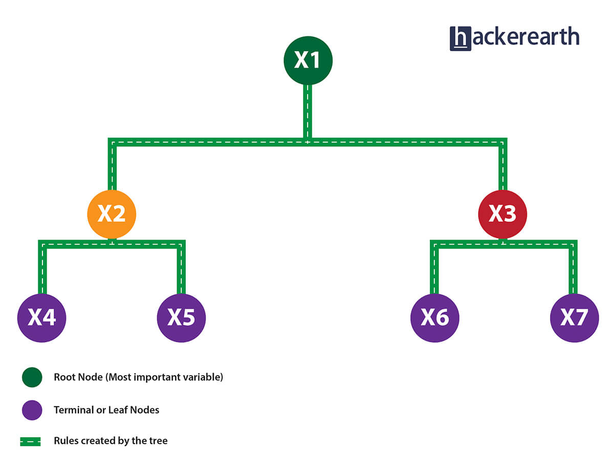
decision tree explaining

1. Given a data frame (n x p), a tree stratifies or partitions the data based on rules (if-else). Yes, a tree creates rules. These rules divide the data set into distinct and non-overlapping regions. These rules are determined by a variable's contribution to the homogeneity or pureness of the resultant child nodes (X2, X3).

2. In the image above, the variable X1 resulted in highest homogeneity in child nodes, hence it became the root node. A variable at root node is also seen as the most important variable in the data set.

3. But how is this homogeneity or pureness determined? In other words, how does the tree decide at which variable to split?

  • In regression trees (where the output is predicted using the mean of observations in the terminal nodes), the splitting decision is based on minimizing RSS. The variable which leads to the greatest possible reduction in RSS is chosen as the root node. The tree splitting takes a top-down greedy approach, also known as recursive binary splitting. We call it "greedy" because the algorithm cares to make the best split at the current step rather than saving a split for better results on future nodes.
  • In classification trees (where the output is predicted using mode of observations in the terminal nodes), the splitting decision is based on the following methods:
    • Gini Index - It's a measure of node purity. If the Gini index takes on a smaller value, it suggests that the node is pure. For a split to take place, the Gini index for a child node should be less than that for the parent node.
    • Entropy - Entropy is a measure of node impurity. For a binary class (a, b), the formula to calculate it is shown below. Entropy is maximum at p = 0.5. For p(X=a)=0.5 or p(X=b)=0.5 means a new observation has a 50%-50% chance of getting classified in either class. The entropy is minimum when the probability is 0 or 1.

Entropy = - p(a)*log(p(a)) - p(b)*log(p(b))
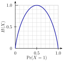
entropy curve

In a nutshell, every tree attempts to create rules in such a way that the resultant terminal nodes could be as pure as possible. Higher the purity, lesser the uncertainty to make the decision.

But a decision tree suffers from high variance. "High Variance" means getting high prediction error on unseen data. We can overcome the variance problem by using more data for training. But since the data set available is limited to us, we can use resampling techniques like bagging and random forest to generate more data.

Building many decision trees results in a forest. A random forest works the following way:

  1. First, it uses the Bagging (Bootstrap Aggregating) algorithm to create random samples. Given a data set D1 (n rows and p columns), it creates a new dataset (D2) by sampling n cases at random with replacement from the original data. About 1/3 of the rows from D1 are left out, known as Out of Bag (OOB) samples.
  2. Then, the model trains on D2. OOB sample is used to determine unbiased estimate of the error.
  3. Out of p columns, P ≪ p columns are selected at each node in the data set. The P columns are selected at random. Usually, the default choice of P is p/3 for regression tree and √p for classification tree.
  4. pruning decision trees Unlike a tree, no pruning takes place in random forest; i.e., each tree is grown fully. In decision trees, pruning is a method to avoid overfitting. Pruning means selecting a subtree that leads to the lowest test error rate. We can use cross-validation to determine the test error rate of a subtree.
  5. Several trees are grown and the final prediction is obtained by averaging (for regression) or majority voting (for classification).

Each tree is grown on a different sample of original data. Since random forest has the feature to calculate OOB error internally, cross-validation doesn't make much sense in random forest.

What is the difference between Bagging and Random Forest?

Many a time, we fail to ascertain that bagging is not the same as random forest. To understand the difference, let's see how bagging works:

  1. It creates randomized samples of the dataset (just like random forest) and grows trees on a different sample of the original data. The remaining 1/3 of the sample is used to estimate unbiased OOB error.
  2. It considers all the features at a node (for splitting).
  3. Once the trees are fully grown, it uses averaging or voting to combine the resultant predictions.

Aren't you thinking, "If both the algorithms do the same thing, what is the need for random forest? Couldn't we have accomplished our task with bagging?" NO!

The need for random forest surfaced after discovering that the bagging algorithm results in correlated trees when faced with a dataset having strong predictors. Unfortunately, averaging several highly correlated trees doesn't lead to a large reduction in variance.

But how do correlated trees emerge? Good question! Let's say a dataset has a very strong predictor, along with other moderately strong predictors. In bagging, a tree grown every time would consider the very strong predictor at its root node, thereby resulting in trees similar to each other.

The main difference between random forest and bagging is that random forest considers only a subset of predictors at a split. This results in trees with different predictors at the top split, thereby resulting in decorrelated trees and more reliable average output. That's why we say random forest is robust to correlated predictors.

Advantages and Disadvantages of Random Forest

Advantages are as follows:

  1. It is robust to correlated predictors.
  2. It is used to solve both regression and classification problems.
  3. It can also be used to solve unsupervised ML problems.
  4. It can handle thousands of input variables without variable selection.
  5. It can be used as a feature selection tool using its variable importance plot.
  6. It takes care of missing data internally in an effective manner.

Disadvantages are as follows:

  1. The Random Forest model is difficult to interpret.
  2. It tends to return erratic predictions for observations out of the range of training data. For example, if the training data contains a variable x ranging from 30 to 70, and the test data has x = 200, random forest would give an unreliable prediction.
  3. It can take longer than expected to compute a large number of trees.

Solving a Problem (Parameter Tuning)

Let's take a dataset to compare the performance of bagging and random forest algorithms. Along the way, I'll also explain important parameters used for parameter tuning. In R, we'll use MLR and data.table packages to do this analysis.

I've taken the Adult dataset from the UCI machine learning repository. You can download the data from here.

This dataset presents a binary classification problem to solve. Given a set of features, we need to predict if a person's salary is <=50K or >=50K. Since the given data isn't well structured, we'll need to make some modification while reading the dataset.

# set working directory
path <- "~/December 2016/RF_Tutorial"
setwd(path)
# Set working directory
path <- "~/December 2016/RF_Tutorial"
setwd(path)

# Load libraries
library(data.table)
library(mlr)
library(h2o)

# Set variable names
setcol <- c("age",
            "workclass",
            "fnlwgt",
            "education",
            "education-num",
            "marital-status",
            "occupation",
            "relationship",
            "race",
            "sex",
            "capital-gain",
            "capital-loss",
            "hours-per-week",
            "native-country",
            "target")

# Load data
train <- read.table("adultdata.txt", header = FALSE, sep = ",", 
                    col.names = setcol, na.strings = c(" ?"), stringsAsFactors = FALSE)
test <- read.table("adulttest.txt", header = FALSE, sep = ",", 
                   col.names = setcol, skip = 1, na.strings = c(" ?"), stringsAsFactors = FALSE)

After we've loaded the dataset, first we'll set the data class to data.table. data.table is the most powerful R package made for faster data manipulation.


>setDT(train)
>setDT(test)

Now, we'll quickly look at given variables, data dimensions, etc.


>dim(train)
>dim(test)
>str(train)
>str(test)

As seen from the output above, we can derive the following insights:

  1. The train dataset has 32,561 rows and 15 columns.
  2. The test dataset has 16,281 rows and 15 columns.
  3. Variable target is the dependent variable.
  4. The target variable in train and test data is different. We'll need to match them.
  5. All character variables have a leading whitespace which can be removed.

We can check missing values using:

# Check missing values in train and test datasets
>table(is.na(train))
# Output:
#  FALSE   TRUE 
#  484153  4262

>sapply(train, function(x) sum(is.na(x)) / length(x)) * 100

table(is.na(test))
# Output:
#  FALSE  TRUE 
#  242012 2203

>sapply(test, function(x) sum(is.na(x)) / length(x)) * 100

As seen above, both train and test datasets have missing values. The sapply function is quite handy when it comes to performing column computations. Above, it returns the percentage of missing values per column.

Now, we'll preprocess the data to prepare it for training. In R, random forest internally takes care of missing values using mean/mode imputation. Practically speaking, sometimes it takes longer than expected for the model to run.

Therefore, in order to avoid waiting time, let's impute the missing values using median/mode imputation method; i.e., missing values in the integer variables will be imputed with median and in the factor variables with mode (most frequent value).

We'll use the impute function from the mlr package, which is enabled with several unique methods for missing value imputation:

# Impute missing values
>imp1 <- impute(data = train, target = "target", 
              classes = list(integer = imputeMedian(), factor = imputeMode()))

>imp2 <- impute(data = test, target = "target", 
              classes = list(integer = imputeMedian(), factor = imputeMode()))

# Assign the imputed data back to train and test
>train <- imp1$data
>test <- imp2$data

Being a binary classification problem, you are always advised to check if the data is imbalanced or not. We can do it in the following way:

# Check class distribution in train and test datasets
setDT(train)[, .N / nrow(train), target]
# Output:
#    target     V1
# 1: <=50K   0.7591904
# 2: >50K    0.2408096

setDT(test)[, .N / nrow(test), target]
# Output:
#    target     V1
# 1: <=50K.  0.7637737
# 2: >50K.   0.2362263

If you observe carefully, the value of the target variable is different in test and train. For now, we can consider it a typo error and correct all the test values. Also, we see that 75% of people in the train data have income <=50K. Imbalanced classification problems are known to be more skewed with a binary class distribution of 90% to 10%. Now, let's proceed and clean the target column in test data.

# Clean trailing character in test target values
test[, target := substr(target, start = 1, stop = nchar(target) - 1)]

We've used the substr function to return the substring from a specified start and end position. Next, we'll remove the leading whitespaces from all character variables. We'll use the str_trim function from the stringr package.

> library(stringr)
> char_col <- colnames(train)[sapply(train, is.character)]
> for(i in char_col)
>     set(train, j = i, value = str_trim(train[[i]], side = "left"))

Using sapply function, we've extracted the column names which have character class. Then, using a simple for - set loop we traversed all those columns and applied the str_trim function.

Before we start model training, we should convert all character variables to factor. MLR package treats character class as unknown.


> fact_col <- colnames(train)[sapply(train,is.character)]
>for(i in fact_col)
			set(train,j=i,value = factor(train[[i]]))
>for(i in fact_col)
	     set(test,j=i,value = factor(test[[i]]))

Let's start with modeling now. MLR package has its own function to convert data into a task, build learners, and optimize learning algorithms. I suggest you stick to the modeling structure described below for using MLR on any data set.

#create a task
> traintask <- makeClassifTask(data = train,target = "target")
> testtask <- makeClassifTask(data = test,target = "target")

#create learner > bag <- makeLearner("classif.rpart",predict.type = "response") > bag.lrn <- makeBaggingWrapper(learner = bag,bw.iters = 100,bw.replace = TRUE)

I've set up the bagging algorithm which will grow 100 trees on randomized samples of data with replacement. To check the performance, let's set up a validation strategy too:

#set 5 fold cross validation
> rdesc <- makeResampleDesc("CV", iters = 5L)

For faster computation, we'll use parallel computation backend. Make sure your machine / laptop doesn't have many programs running in the background.

#set parallel backend (Windows)
> library(parallelMap)
> library(parallel)
> parallelStartSocket(cpus = detectCores())
>

For linux users, the function parallelStartMulticore(cpus = detectCores()) will activate parallel backend. I've used all the cores here.

r <- resample(learner = bag.lrn,
              task = traintask,
              resampling = rdesc,
              measures = list(tpr, fpr, fnr, fpr, acc),
              show.info = T)

#[Resample] Result: 
# tpr.test.mean = 0.95,
# fnr.test.mean = 0.0505,
# fpr.test.mean = 0.487,
# acc.test.mean = 0.845

Being a binary classification problem, I've used the components of confusion matrix to check the model's accuracy. With 100 trees, bagging has returned an accuracy of 84.5%, which is way better than the baseline accuracy of 75%. Let's now check the performance of random forest.

#make randomForest learner
> rf.lrn <- makeLearner("classif.randomForest")
> rf.lrn$par.vals <- list(ntree = 100L,
                          importance = TRUE)

> r <- resample(learner = rf.lrn,
                task = traintask,
                resampling = rdesc,
                measures = list(tpr, fpr, fnr, fpr, acc),
                show.info = T)

# Result:
# tpr.test.mean = 0.996,
# fpr.test.mean = 0.72,
# fnr.test.mean = 0.0034,
# acc.test.mean = 0.825

On this data set, random forest performs worse than bagging. Both used 100 trees and random forest returns an overall accuracy of 82.5 %. An apparent reason being that this algorithm is messing up classifying the negative class. As you can see, it classified 99.6% of the positive classes correctly, which is way better than the bagging algorithm. But it incorrectly classified 72% of the negative classes.

Internally, random forest uses a cutoff of 0.5; i.e., if a particular unseen observation has a probability higher than 0.5, it will be classified as <=50K. In random forest, we have the option to customize the internal cutoff. As the false positive rate is very high now, we'll increase the cutoff for positive classes (<=50K) and accordingly reduce it for negative classes (>=50K). Then, train the model again.

#set cutoff
> rf.lrn$par.vals <- list(ntree = 100L,
                          importance = TRUE,
                          cutoff = c(0.75, 0.25))

> r <- resample(learner = rf.lrn,
                task = traintask,
                resampling = rdesc,
                measures = list(tpr, fpr, fnr, fpr, acc),
                show.info = T)

#Result: 
# tpr.test.mean = 0.934,
# fpr.test.mean = 0.43,
# fnr.test.mean = 0.0662,
# acc.test.mean = 0.846

As you can see, we've improved the accuracy of the random forest model by 2%, which is slightly higher than that for the bagging model. Now, let's try and make this model better.

Parameter Tuning: Mainly, there are three parameters in the random forest algorithm which you should look at (for tuning):

  • ntree - As the name suggests, the number of trees to grow. Larger the tree, it will be more computationally expensive to build models.
  • mtry - It refers to how many variables we should select at a node split. Also as mentioned above, the default value is p/3 for regression and sqrt(p) for classification. We should always try to avoid using smaller values of mtry to avoid overfitting.
  • nodesize - It refers to how many observations we want in the terminal nodes. This parameter is directly related to tree depth. Higher the number, lower the tree depth. With lower tree depth, the tree might even fail to recognize useful signals from the data.

Let get to the playground and try to improve our model's accuracy further. In MLR package, you can list all tuning parameters a model can support using:

> getParamSet(rf.lrn)

# set parameter space
params <- makeParamSet(
    makeIntegerParam("mtry", lower = 2, upper = 10),
    makeIntegerParam("nodesize", lower = 10, upper = 50)
)

# set validation strategy
rdesc <- makeResampleDesc("CV", iters = 5L)

# set optimization technique
ctrl <- makeTuneControlRandom(maxit = 5L)

# start tuning
> tune <- tuneParams(learner = rf.lrn,
                     task = traintask,
                     resampling = rdesc,
                     measures = list(acc),
                     par.set = params,
                     control = ctrl,
                     show.info = T)

[Tune] Result: mtry=2; nodesize=23 : acc.test.mean=0.858

After tuning, we have achieved an overall accuracy of 85.8%, which is better than our previous random forest model. This way you can tweak your model and improve its accuracy.

I'll leave you here. The complete code for this analysis can be downloaded from Github.

Summary

Don't stop here! There is still a huge scope for improvement in this model. Cross validation accuracy is generally more optimistic than true test accuracy. To make a prediction on the test set, minimal data preprocessing on categorical variables is required. Do it and share your results in the comments below.

My motive to create this tutorial is to get you started using the random forest model and some techniques to improve model accuracy. For better understanding, I suggest you read more on confusion matrix. In this article, I've explained the working of decision trees, random forest, and bagging.

Did I miss out anything? Do share your knowledge and let me know your experience while solving classification problems in comments below.

Subscribe to The HackerEarth Blog

Get expert tips, hacks, and how-tos from the world of tech recruiting to stay on top of your hiring!

Author
Manish Saraswat
Calendar Icon
December 14, 2016
Timer Icon
15 min read
Share

Hire top tech talent with our recruitment platform

Access Free Demo
Related reads

Discover more articles

Gain insights to optimize your developer recruitment process.

The Mobile Dev Hiring Landscape Just Changed

Revolutionizing Mobile Talent Hiring: The HackerEarth AdvantageThe demand for mobile applications is exploding, but finding and verifying developers with proven, real-world skills is more difficult than ever. Traditional assessment methods often fall short, failing to replicate the complexities of modern mobile development.Introducing a New Era in Mobile AssessmentAt HackerEarth, we're...

Revolutionizing Mobile Talent Hiring: The HackerEarth Advantage

The demand for mobile applications is exploding, but finding and verifying developers with proven, real-world skills is more difficult than ever. Traditional assessment methods often fall short, failing to replicate the complexities of modern mobile development.

Introducing a New Era in Mobile Assessment

At HackerEarth, we're closing this critical gap with two groundbreaking features, seamlessly integrated into our Full Stack IDE:

Article content

Now, assess mobile developers in their true native environment. Our enhanced Full Stack questions now offer full support for both Java and Kotlin, the core languages powering the Android ecosystem. This allows you to evaluate candidates on authentic, real-world app development skills, moving beyond theoretical knowledge to practical application.

Article content

Say goodbye to setup drama and tool-switching. Candidates can now build, test, and debug Android and React Native applications directly within the browser-based IDE. This seamless, in-browser experience provides a true-to-life evaluation, saving valuable time for both candidates and your hiring team.

Assess the Skills That Truly Matter

With native Android support, your assessments can now delve into a candidate's ability to write clean, efficient, and functional code in the languages professional developers use daily. Kotlin's rapid adoption makes proficiency in it a key indicator of a forward-thinking candidate ready for modern mobile development.

Breakup of Mobile development skills ~95% of mobile app dev happens through Java and Kotlin
This chart illustrates the importance of assessing proficiency in both modern (Kotlin) and established (Java) codebases.

Streamlining Your Assessment Workflow

The integrated mobile emulator fundamentally transforms the assessment process. By eliminating the friction of fragmented toolchains and complex local setups, we enable a faster, more effective evaluation and a superior candidate experience.

Old Fragmented Way vs. The New, Integrated Way
Visualize the stark difference: Our streamlined workflow removes technical hurdles, allowing candidates to focus purely on demonstrating their coding and problem-solving abilities.

Quantifiable Impact on Hiring Success

A seamless and authentic assessment environment isn't just a convenience, it's a powerful catalyst for efficiency and better hiring outcomes. By removing technical barriers, candidates can focus entirely on demonstrating their skills, leading to faster submissions and higher-quality signals for your recruiters and hiring managers.

A Better Experience for Everyone

Our new features are meticulously designed to benefit the entire hiring ecosystem:

For Recruiters & Hiring Managers:

  • Accurately assess real-world development skills.
  • Gain deeper insights into candidate proficiency.
  • Hire with greater confidence and speed.
  • Reduce candidate drop-off from technical friction.

For Candidates:

  • Enjoy a seamless, efficient assessment experience.
  • No need to switch between different tools or manage complex setups.
  • Focus purely on showcasing skills, not environment configurations.
  • Work in a powerful, professional-grade IDE.

Unlock a New Era of Mobile Talent Assessment

Stop guessing and start hiring the best mobile developers with confidence. Explore how HackerEarth can transform your tech recruiting.

Vibe Coding: Shaping the Future of Software

A New Era of CodeVibe coding is a new method of using natural language prompts and AI tools to generate code. I have seen firsthand that this change makes software more accessible to everyone. In the past, being able to produce functional code was a strong advantage for developers. Today,...

A New Era of Code

Vibe coding is a new method of using natural language prompts and AI tools to generate code. I have seen firsthand that this change makes software more accessible to everyone. In the past, being able to produce functional code was a strong advantage for developers. Today, when code is produced quickly through AI, the true value lies in designing, refining, and optimizing systems. Our role now goes beyond writing code; we must also ensure that our systems remain efficient and reliable.

From Machine Language to Natural Language

I recall the early days when every line of code was written manually. We progressed from machine language to high-level programming, and now we are beginning to interact with our tools using natural language. This development does not only increase speed but also changes how we approach problem solving. Product managers can now create working demos in hours instead of weeks, and founders have a clearer way of pitching their ideas with functional prototypes. It is important for us to rethink our role as developers and focus on architecture and system design rather than simply on typing c

The Promise and the Pitfalls

I have experienced both sides of vibe coding. In cases where the goal was to build a quick prototype or a simple internal tool, AI-generated code provided impressive results. Teams have been able to test new ideas and validate concepts much faster. However, when it comes to more complex systems that require careful planning and attention to detail, the output from AI can be problematic. I have seen situations where AI produces large volumes of code that become difficult to manage without significant human intervention.

AI-powered coding tools like GitHub Copilot and AWS’s Q Developer have demonstrated significant productivity gains. For instance, at the National Australia Bank, it’s reported that half of the production code is generated by Q Developer, allowing developers to focus on higher-level problem-solving . Similarly, platforms like Lovable or Hostinger Horizons enable non-coders to build viable tech businesses using natural language prompts, contributing to a shift where AI-generated code reduces the need for large engineering teams. However, there are challenges. AI-generated code can sometimes be verbose or lack the architectural discipline required for complex systems. While AI can rapidly produce prototypes or simple utilities, building large-scale systems still necessitates experienced engineers to refine and optimize the code.​

The Economic Impact

The democratization of code generation is altering the economic landscape of software development. As AI tools become more prevalent, the value of average coding skills may diminish, potentially affecting salaries for entry-level positions. Conversely, developers who excel in system design, architecture, and optimization are likely to see increased demand and compensation.​
Seizing the Opportunity

Vibe coding is most beneficial in areas such as rapid prototyping and building simple applications or internal tools. It frees up valuable time that we can then invest in higher-level tasks such as system architecture, security, and user experience. When used in the right context, AI becomes a helpful partner that accelerates the development process without replacing the need for skilled engineers.

This is revolutionizing our craft, much like the shift from machine language to assembly to high-level languages did in the past. AI can churn out code at lightning speed, but remember, “Any fool can write code that a computer can understand. Good programmers write code that humans can understand.” Use AI for rapid prototyping, but it’s your expertise that transforms raw output into robust, scalable software. By honing our skills in design and architecture, we ensure our work remains impactful and enduring. Let’s continue to learn, adapt, and build software that stands the test of time.​

Ready to streamline your recruitment process? Get a free demo to explore cutting-edge solutions and resources for your hiring needs.

Guide to Conducting Successful System Design Interviews in 2025

What is Systems Design?Systems Design is an all encompassing term which encapsulates both frontend and backend components harmonized to define the overall architecture of a product.Designing robust and scalable systems requires a deep understanding of application, architecture and their underlying components like networks, data, interfaces and modules.Systems Design, in its...

What is Systems Design?

Systems Design is an all encompassing term which encapsulates both frontend and backend components harmonized to define the overall architecture of a product.

Designing robust and scalable systems requires a deep understanding of application, architecture and their underlying components like networks, data, interfaces and modules.

Systems Design, in its essence, is a blueprint of how software and applications should work to meet specific goals. The multi-dimensional nature of this discipline makes it open-ended – as there is no single one-size-fits-all solution to a system design problem.

What is a System Design Interview?

Conducting a System Design interview requires recruiters to take an unconventional approach and look beyond right or wrong answers. Recruiters should aim for evaluating a candidate’s ‘systemic thinking’ skills across three key aspects:

How they navigate technical complexity and navigate uncertainty
How they meet expectations of scale, security and speed
How they focus on the bigger picture without losing sight of details

This assessment of the end-to-end thought process and a holistic approach to problem-solving is what the interview should focus on.

What are some common topics for a System Design Interview

System design interview questions are free-form and exploratory in nature where there is no right or best answer to a specific problem statement. Here are some common questions:

How would you approach the design of a social media app or video app?

What are some ways to design a search engine or a ticketing system?

How would you design an API for a payment gateway?

What are some trade-offs and constraints you will consider while designing systems?

What is your rationale for taking a particular approach to problem solving?

Usually, interviewers base the questions depending on the organization, its goals, key competitors and a candidate’s experience level.

For senior roles, the questions tend to focus on assessing the computational thinking, decision making and reasoning ability of a candidate. For entry level job interviews, the questions are designed to test the hard skills required for building a system architecture.

The Difference between a System Design Interview and a Coding Interview

If a coding interview is like a map that takes you from point A to Z – a systems design interview is like a compass which gives you a sense of the right direction.

Here are three key difference between the two:

Coding challenges follow a linear interviewing experience i.e. candidates are given a problem and interaction with recruiters is limited. System design interviews are more lateral and conversational, requiring active participation from interviewers.

Coding interviews or challenges focus on evaluating the technical acumen of a candidate whereas systems design interviews are oriented to assess problem solving and interpersonal skills.

Coding interviews are based on a right/wrong approach with ideal answers to problem statements while a systems design interview focuses on assessing the thought process and the ability to reason from first principles.

How to Conduct an Effective System Design Interview

One common mistake recruiters make is that they approach a system design interview with the expectations and preparation of a typical coding interview.
Here is a four step framework technical recruiters can follow to ensure a seamless and productive interview experience:

Step 1: Understand the subject at hand

  • Develop an understanding of basics of system design and architecture
  • Familiarize yourself with commonly asked systems design interview questions
  • Read about system design case studies for popular applications
  • Structure the questions and problems by increasing magnitude of difficulty

Step 2: Prepare for the interview

  • Plan the extent of the topics and scope of discussion in advance
  • Clearly define the evaluation criteria and communicate expectations
  • Quantify constraints, inputs, boundaries and assumptions
  • Establish the broader context and a detailed scope of the exercise

Step 3: Stay actively involved

  • Ask follow-up questions to challenge a solution
  • Probe candidates to gauge real-time logical reasoning skills
  • Make it a conversation and take notes of important pointers and outcomes
  • Guide candidates with hints and suggestions to steer them in the right direction

Step 4: Be a collaborator

  • Encourage candidates to explore and consider alternative solutions
  • Work with the candidate to drill the problem into smaller tasks
  • Provide context and supporting details to help candidates stay on track
  • Ask follow-up questions to learn about the candidate’s experience

Technical recruiters and hiring managers should aim for providing an environment of positive reinforcement, actionable feedback and encouragement to candidates.

Evaluation Rubric for Candidates

Facilitate Successful System Design Interview Experiences with FaceCode

FaceCode, HackerEarth’s intuitive and secure platform, empowers recruiters to conduct system design interviews in a live coding environment with HD video chat.

FaceCode comes with an interactive diagram board which makes it easier for interviewers to assess the design thinking skills and conduct communication assessments using a built-in library of diagram based questions.

With FaceCode, you can combine your feedback points with AI-powered insights to generate accurate, data-driven assessment reports in a breeze. Plus, you can access interview recordings and transcripts anytime to recall and trace back the interview experience.

Learn how FaceCode can help you conduct system design interviews and boost your hiring efficiency.

Top Products

Explore HackerEarth’s top products for Hiring & Innovation

Discover powerful tools designed to streamline hiring, assess talent efficiently, and run seamless hackathons. Explore HackerEarth’s top products that help businesses innovate and grow.
Frame
Hackathons
Engage global developers through innovation
Arrow
Frame 2
Assessments
AI-driven advanced coding assessments
Arrow
Frame 3
FaceCode
Real-time code editor for effective coding interviews
Arrow
Frame 4
L & D
Tailored learning paths for continuous assessments
Arrow
Get A Free Demo