
Introduction
Human learners appear to have inherent ways to transfer knowledge between tasks. That is, we recognize and apply relevant knowledge from previous learning experience when we encounter new tasks. The more related a new task is to our previous experience, the more easily we can master it.
Transfer learning involves the approach in which knowledge learned in one or more source tasks is transferred and used to improve the learning of a related target task. While most machine learning algorithms are designed to address single tasks, the development of algorithms that facilitate transfer learning is a topic of ongoing interest in the machine-learning community.
Why transfer learning ?
Many deep neural networks trained on natural images exhibit a curious phenomenon in common: on the first layer they learn features similar to Gabor filters and color blobs. Such first-layer features appear not to specific to a particular dataset or task but are general in that they are applicable to many datasets and tasks. As finding these standard features on the first layer seems to occur regardless of the exact cost function and natural image dataset, we call these first-layer features general. For example, in a network with an N-dimensional softmax output layer that has been successfully trained towards a supervised classification objective, each output unit will be specific to a particular class. We thus call the last-layer features specific.
In transfer learning we first train a base network on a base dataset and task, and then we repurpose the learned features, or transfer them, to a second target network to be trained on a target dataset and task. This process will tend to work if the features are general, that is, suitable to both base and target tasks, instead of being specific to the base task.
In practice, very few people train an entire Convolutional Network from scratch because it is relatively rare to have a dataset of sufficient size. Instead, it is common to pre-train a ConvNet on a very large dataset (e.g. ImageNet, which contains 1.2 million images with 1000 categories), and then use the ConvNet either as an initialization or a fixed feature extractor for the task of interest.
Transfer learning scenarios
Depending on both the size of the new dataset and the similarity of the new dataset to the original dataset, the approach for using transfer learning will be different. Keeping in mind that ConvNet features are more generic in the early layers and more original-dataset specific in the later layers, here are some common rules of thumb for navigating the four major scenarios:
-
The target dataset is small and similar to the base training dataset.
Since the target dataset is small, it is not a good idea to fine-tune the ConvNet due to the risk of overfitting. Since the target data is similar to the base data, we expect higher-level features in the ConvNet to be relevant to this dataset as well. Hence, we:- Remove the fully connected layers near the end of the pretrained base ConvNet
- Add a new fully connected layer that matches the number of classes in the target dataset
- Randomize the weights of the new fully connected layer and freeze all the weights from the pre-trained network
- Train the network to update the weights of the new fully connected layers
-
The target dataset is large and similar to the base training dataset.
Since the target dataset is large, we have more confidence that we won\u2019t overfit if we try to fine-tune through the full network. Therefore, we:- Remove the last fully connected layer and replace with the layer matching the number of classes in the target dataset
- Randomly initialize the weights in the new fully connected layer
- Initialize the rest of the weights using the pre-trained weights, i.e., unfreeze the layers of the pre-trained network
- Retrain the entire neural network
-
The target dataset is small and different from the base training dataset.
Since the data is small, overfitting is a concern. Hence, we train only the linear layers. But as the target dataset is very different from the base dataset, the higher level features in the ConvNet would not be of any relevance to the target dataset. So, the new network will only use the lower level features of the base ConvNet. To implement this scheme, we:- Remove most of the pre-trained layers near the beginning of the ConvNet
- Add to the remaining pre-trained layers new fully connected layers that match the number of classes in the new dataset
- Randomize the weights of the new fully connected layers and freeze all the weights from the pre-trained network
- Train the network to update the weights of the new fully connected layers
-
The target dataset is large and different from the base training dataset.
As the target dataset is large and different from the base dataset, we can train the ConvNet from scratch. However, in practice, it is beneficial to initialize the weights from the pre-trained network and fine-tune them as it might make the training faster. In this condition, the implementation is the same as in case 3.
Transfer learning in Keras
We will be using the Cifar-10 dataset and the keras framework to implement our model. In this post, we will first build a model from scratch and then try to improve it by implementing transfer learning. Before we start to code, let\u2019s discuss the Cifar-10 dataset in brief. Cifar-10 dataset consists of 60,000 32*32 color images in 10 classes, with 6000 images per class. There are 50,000 training images and 10,000 testing images. Let\u2019s begin by importing the dataset. Since this dataset is present in the keras database, we will import it from keras directly.
import numpy as np
from keras.datasets import cifar10

#Load the dataset:
(X_train, y_train), (X_test, y_test) = cifar10.load_data()
Let\u2019s check the shape of the train and test dataset.
print("There are {} train images and {} test images.".format(X_train.shape[0], X_test.shape[0]))
print('There are {} unique classes to predict.'.format(np.unique(y_train).shape[0]))
We, can see that there are 50,000 train images and 10,000 test images with 10 unique classes to predict. Next, we will one-hot label our train and test labels.
#One-hot encoding the labels
num_classes = 10
from keras.utils import np_utils
y_train = np_utils.to_categorical(y_train, num_classes)
y_test = np_utils.to_categorical(y_test, num_classes)
Let\u2019s visualize our training data. We will display the first eight images in the training data.
fig = plt.figure(figsize=(10, 10))

for i in range(1, 9):
    img = X_train[i-1]
    fig.add_subplot(2, 4, i)
    plt.imshow(img)

print(\u2018Shape of each image in the training data: \u2019, X_train.shape[1:])
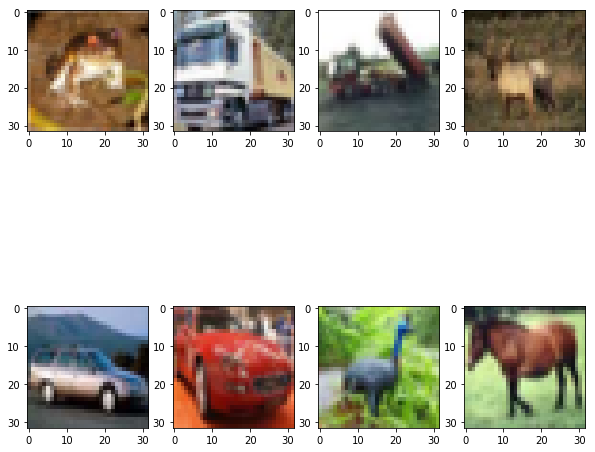
Each image in the dataset is of size: 32*32*3. Now, that we have got an idea of the dataset, let\u2019s build a model from scratch. We will be sticking with the keras framework to build our model as it is easy to understand, but you may use other frameworks also.
#Importing the necessary libraries
from keras.models import Sequential
from keras.layers import Dense, Conv2D, MaxPooling2D
from keras.layers import Dropout, Flatten, GlobalAveragePooling2D

#Building up a Sequential model
model = Sequential()
model.add(Conv2D(32, (3, 3), activation='relu',input_shape = X_train.shape[1:]))
model.add(MaxPooling2D(pool_size=(2, 2)))

model.add(Conv2D(32, (3, 3), activation='relu'))
model.add(MaxPooling2D(pool_size=(2, 2)))

model.add(Conv2D(64, (3, 3), activation='relu'))
model.add(MaxPooling2D(pool_size=(2, 2)))

model.add(GlobalAveragePooling2D())
model.add(Dense(10, activation='softmax'))
model.summary()
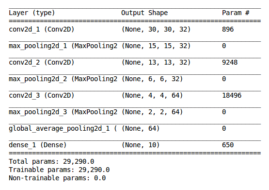
From Fig 2., we can see that our model contains three convolutional layers, each followed by a max pooling layer and finally a Global Average Pooling layer followed by a dense layer with \u2018softmax\u2019 as the activation function. There are a total of 29,290 parameters to train. We will be using \u2018binary cross-entropy\u2019 as the loss function, \u2018adam\u2019 as the optimizer and \u2018accuracy\u2019 as the performance metric.
model.compile(loss='binary_crossentropy', optimizer='adam',
              metrics=['accuracy'])
Finally, we will rescale our data. Rescale is a value by which we will multiply the data such that the resultant values lie in the range (0-1). So, in general, scaling ensures that just because some features are big in magnitude, it doesn\u2019t mean they act as the main features in predicting the label.
X_train_scratch = X_train/255.
X_test_scratch = X_test/255.
Next, we will create a checkpointer to save the weights of the best model (i.e. the model with minimum loss).
#Creating a checkpointer
checkpointer = ModelCheckpoint(filepath='scratchmodel.best.hdf5',
                               verbose=1,save_best_only=True)
Finally, we will fit the model to the training data points and labels. We will split the whole training data in batches of 32 and train the model for 10 epochs. We will use be 20 percent of our training data as our validation data. Hence, we will train the model on 10000 samples and validate of 10000 samples.
#Fitting the model on the train data and labels.
model.fit(X_train, y_train, batch_size=32, epochs=10,
          verbose=1, callbacks=[checkpointer], validation_split=0.2, shuffle=True)
The best model produces an accuracy of 82.01% on the training samples and 81.96% on the validation samples. Let\u2019s evaluate the performance of the model on the test dataset.
#Evaluate the model on the test data
score = model.evaluate(X_test, y_test)

#Accuracy on test data
print('Accuracy on the Test Images: ', score[1])
So, our CNN model produces an accuracy of 82% on the test dataset. That\u2019s great, but can we do better. Let\u2019s implement transfer learning and check if we can improve the model. We will be using the Resnet50 model, pre-trained on the \u2018Imagenet weights\u2019 to implement transfer learning. We are using ResNet50 model but may use other models (VGG16, VGG19, InceptionV3, etc.) also.
#Importing the ResNet50 model
from keras.applications.resnet50 import ResNet50, preprocess_input

#Loading the ResNet50 model with pre-trained ImageNet weights
model = ResNet50(weights='imagenet', include_top=False, input_shape=(200, 200, 3))
The Cifar-10 dataset is small and similar to the \u2018ImageNet\u2019 dataset. So, we will remove the fully connected layers of the pre-trained network near the end. To implement this, we set \u2018include_top = False\u2019, while loading the ResNet50 model.
#Reshaping the training data
X_train_new = np.array([imresize(X_train[i], (200, 200, 3)) for i in range(0, len(X_train))]).astype('float32')

#Preprocessing the data, so that it can be fed to the pre-trained ResNet50 model.
resnet_train_input = preprocess_input(X_train_new)

#Creating bottleneck features for the training data
train_features = model.predict(resnet_train_input)

#Saving the bottleneck features
np.savez('resnet_features_train', features=train_features)
As the minimum size of the image that can be supplied to the ResNet50 model is (197 * 197 * 3), we resize our training images to the size (200 * 200 * 3). Next, we preprocess the resized data so that it can be fed to the pre-trained ResNet50 model as input.
Finally, we will use the pre-trained ResNet50 model to create bottleneck features for the training data. Next, we will store these bottleneck features offline because calculating them could be computationally expensive, especially when you're working on the CPU, and we want to only do it once. Note that this prevents us from using data augmentation.
#Reshaping the testing data
X_test_new = np.array([imresize(X_test[i], (200, 200, 3)) for i in range(0, len(X_test))]).astype('float32')

#Preprocessing the data, so that it can be fed to the pre-trained ResNet50 model.
resnet_test_input = preprocess_input(X_test_new)

#Creating bottleneck features for the testing data
test_features = model.predict(resnet_test_input)

#Saving the bottleneck features
np.savez('resnet_features_test', features=test_features)
We will use the same process to create bottleneck features for the testing data. Now, that we have created the bottleneck features, we will supply them as input to a sequential model with newly added fully connected layers that match the number of classes in the Cifar-10 dataset.
model = Sequential()
model.add(GlobalAveragePooling2D(input_shape=train_features.shape[1:]))
model.add(Dropout(0.3))
model.add(Dense(10, activation='softmax'))
model.summary()
Fig 3., represents the model summary of our resnet50 transfer model. We can see that the number of trainable parameters has reduce to 20,490, when compared to the trainable parameters in the CNN model that was build from scratch. Next, we will compile the model. We will use the same \u2018categorical cross-entropy\u2018 as our loss function, \u2018adam\u2019 as our optimizer and \u2018accuracy\u2019 as the performance metric.
model.compile(loss='categorical_crossentropy', optimizer='adam',
              metrics=['accuracy'])
We will create a model checkpointer to save the best model and call the \u2018fit\u2019 method to train the model for 10 epochs. The model trains on 40000 samples and validates on the remaining 10000 samples.
model.fit(train_features, y_train, batch_size=32, epochs=10,
          validation_split=0.2, callbacks=[checkpointer], verbose=1, shuffle=True)
The model produces an accuracy of 90.01% and 88.68% on the training data and validation data respectively. Lastly, we evaluate our model on the test data.
#Evaluate the model on the test data
score  = model.evaluate(test_features, y_test)

#Accuracy on test data
print('Accuracy on the Test Images: ', score[1])
The model produces an accuracy of 88.58% on the test data.
Conclusion
We see that by using pre-trained features, the accuracy of the model jumped from 82% to 88.58% on the test data. Also, the number of trainable parameters in the transfer model is low as compared to our scratch model. Apart from this, the CNN scratch model took around 15 minutes to train on CPU, while the transfer model took less than a minute to train the model. We can conclude that the use of transfer learning not only improves the performance of the model but also is computationally efficient.
Now, the question one may ask is if we can further improve the model, and the answer is yes. We may use techniques such as the following: - Implement data Augmentation - Fine-tuning the optimizer and loss function - Use L1 and L2 regularization - Use a different pre-trained model - Fine-tune the layers of the pre-trained model
Next, I encourage you to apply transfer learning on Cifar-100 dataset (or any other dataset of your choice) and explore the results.
Have anything to say? Feel free to drop your suggestions, recommendations, or concerns in comments below.
References
- Transfer Learning, Lisa Torrey and Jude Shavlik, University of Wisconsin, Madison, WI, USA.
- CS231n Convolutional Neural Networks for Visual Recognition.
- Yosinski J, Clune J, Bengio Y, and Lipson H. How transferable are features in deep neural networks? In Advances in Neural Information Processing Systems 27 (NIPS \u201914), NIPS Foundation, 2014.
- https://www.cs.toronto.edu/~kriz/cifar.html