Introduction

Matrix is a popular math object. It is basically a two-dimensional table of numbers. In this article we’ll look at integer matrices, i.e. tables with integers. This is how matrices are usually pictured:
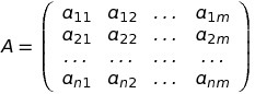
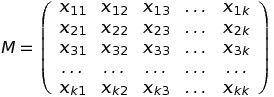
A is the matrix with n rows and m columns. Each integer in A is represented as a_ij: i is the row number (ranging from 1 to n), j is the column number (ranging from 1 to m).

Matrices appear very frequently in computer science, with notable examples being:

1. Adjacency matrix of a graph;
2. Matrix of system of linear equations;
3. Matrices of affine transformations in 3D graphics;
4. Probability vectors, defining probability mass function of discrete random variable.

Even if you don’t know linear algebra (where matrices are heavily studied) or anything like that, I bet you’ve used matrices at least once. This happens every time when you define a 2D-array!
Let’s say you have declared a variable like this (in C++):

int arr[1000][1000];

Then you can write something like this:

for(int i = 0; i < n; i++)
  for(int j = 0; j < n; j++)
    cin >> arr[i][j];

To access 2D-array arr, you use two integers [i][j]. It is exactly the same as with matrix, where you need to specify row number and column number to pinpoint one element. One conclusion from this paragraph: you can represent matrices in code with 2D-arrays.

Surprisingly, in competitive programming matrices can appear too. There are 10 problems with tag “Matrix exponentiation” on HackerEarth (at the time of writing). 8 of them also have tag “Hard”. If you become familiar with matrices and exponentiating them, those problems will become at least “Medium” for you, or even “Easy”!

Matrix multiplication

Consider two matrices:

1. Matrix A have n rows and k columns;
2. Matrix B have k rows and m columns (notice that number of rows in B is the same as number of columns in A).

Then we define operation:
C = A * B (matrix multiplication)

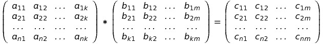
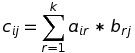
such that C is a matrix with n rows and m columns, and each element of C should be computed by the following formula:

The meaning of matrix multiplication is different for different usage of matrices, so it is OK if you still have no idea how multiplication could be useful.

Several things to notice:

1. Matrix C has the same number of rows as A, and the same number of columns as B;
2. Matrix C has n * m elements, each element is computed in k steps with given formula => we can obtain C in O(n * m * k), given A and B;
3. If n = m = k (i.e. both A and B have n rows and n columns), then C has n rows and n columns, and can be computed in O(n³).

Here are some useful properties of matrix multiplication:

1. It is not commutative: A * B ≠ B * A in general case;
2. It is associative: A * B * C = (A * B) * C = A * (B * C) in case A * B * C exists;
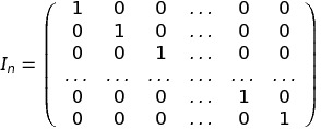
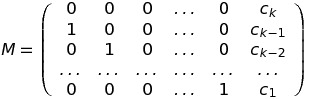
3. If you have matrix with n rows and n columns, then multiplying it by I_n gives the same matrix, i. e. I_n * A = A * I_n = A. I_n is a matrix with n rows and n columns of such form:

Matrix exponentiation

Suppose you have a matrix A with n rows and n columns (we’ll call such matrices “square matrix of size n”). We can define matrix exponentiation as:
A^x = A * A * A * … * A (x times)
with special case of x = 0:
A⁰ = I_n
Here x is non-negative integer (i. e. 0, 1, 2, 3, …). Don’t worry if this operation seem meaningless to you. Let’s now analyse how fast we can compute A^x, given A and x.

The brute-force solution would be (written in pseudo code):

function matrix_power_naive(A, x):
  result = I_n
  for i = 1..x:
    result = result * A
  return result

It runs in Θ(n³ * x): we do x matrix multiplications on square matrices of size n, and each multiplication runs in Θ(n³).

We can do better! Let’s choose x = 75 as an example. Write down binary representation of x:
75₁₀ = 1001011₂ => 75 = 2⁰ + 2¹ + 2³ + 2⁶ = 1 + 2 + 8 + 64.
Now we can rewrite A^x as
A⁷⁵ = A¹ * A² * A⁸ * A⁶⁴. There are a lot less multiples, don’t you think? We had 75 of them, now we’ve got only 4, which is a number of 1’s in binary representation of our x.
And it turns out, we can find A^2r really fast for any r:
A²⁰ = A¹ = A (zero steps)
A²¹ = A^{20 * 2} = A^{20 + 20} = A²⁰ * A²⁰ (one multiplication - n³ steps)
A²² = A^{21 * 2} = A^{21 + 21} = A²¹ * A²¹ (one multiplication - 2 * n³ steps)
… (computations happen) ...
A^2r = A^{2r - 1 * 2} = A^{2r - 1 + 2r - 1} = A^{2r - 1} * A^{2r - 1} (one multiplication - r * n³ steps)
Therefore, we can find A^2r in O(r * n³) time, given A and r. Notice, however, that r = O(log(x)), because we compute A^2r only when there is r’th bit is set to 1 in binary representation of x, and length of binary representation of x is not more than log₂(x) + 1.

So, for x = 75 we compute A², A⁴, A⁸, A¹⁶, A³², A⁶⁴ (that’s the fastest way we can get A⁶⁴) in 6 * n³ steps, then perform 4 multiplications (I_n * A¹ * A² * A⁸ * A⁶⁴) in 4 * n³ steps. In total, this gets us to 10 * n³ steps for computing A⁷⁵, instead of 75 * n³ steps with brute force.

We could implement this new idea in general (for any x) in the following way:

function matrix_power_smart(A, x):
  result = I_n
  r = 0
  cur_a = A
  while 2^r <= x:
    if r’th bit is set in x:
      result = result * cur_a
    r += 1
    cur_a = cur_a * cur_a
  return result

Here, on every step of the while loop, cur_a = A^2r.
While the above code works, there is a more conventional way of implementing this algorithm. Instead of incrementing r, we will strip the 0’th bit from x on every iteration. And instead of checking if r’th bit is set, we must check if 0’th bit is set in x. Also, instead of having variable cur_a, we will multiply A by itself in-place.

Here is the implementation:

function matrix_power_final(A, x):
  result = I_n
  while x > 0:
    if x % 2 == 1:
      result = result * A
    A = A * A
    x = x / 2
  return result

Major conclusion here: we can find A^x for any integer x in O(n³ * log₂x) time.

Applications of matrix exponentiation

Finding N’th Fibonacci number

1. F₀ = F₁ = 1;
2. F_i = F_{i - 1} + F_{i - 2} for i ≥ 2.

We want to find F_N modulo 1000000007, where N can be up to 10¹⁸.

The first thing that comes to mind is to run a for loop, according to the definition:

function fibonacci_definition(N):
  if N <= 1:
    return 1
  x = 1
  y = 1
  for i = 0..N-2:
    next_y = (x + y) mod 1000000007
    x = y
    y = next_y
  return y

After i’th iteration of for loop, we maintain x = F_{i + 1} and y = F_{i + 2}. As the last iteration is N-2’th, we get y = F_{N - 2 + 2} = F_N when we return from the function.
The running time of this loop is clearly O(N). This can work in reasonable time for N up to 10⁹. If we want N up to 10¹⁸, we have to switch to a faster approach.

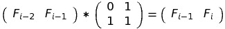
Here is when matrices get involved. Suppose we have a vector (matrix with one row and several columns) of (F_{i - 2}, F_{i - 1}) and we want to multiply it by some matrix, so that we get (F_{i - 1}, F_i). Let’s call this matrix M:

Two questions arise immediately:

1. What are the dimensions of M?
2. What are exact values in M?

We can answer them, using the definition of matrix multiplication:

1. The size. We multiply the (F_{i - 2}, F_{i - 1}), which has 1 row and 2 columns, by M. The result is (F_{i - 1}, F_i), which has 1 row and 2 columns.
   By definition, if we multiply a matrix with n rows and k columns by a matrix with k rows and m columns, we get a matrix with n rows and m columns.
   In our case, n = 1, k = 2 (number of rows and columns of (F_{i - 2}, F_{i - 1})), and m = 2 (number of columns in the resulting (F_{i - 1}, F_i)).
   Therefore, M has k = 2 rows and m = 2 columns.
2. Values. We now know that M has 2 rows and 2 columns, 4 values overall. Let’s denote them by letters, as we usually do with unknown variables:
   
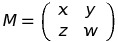
   We want to find x, y, z and w. Let’s see what we get, if we multiply (F_{i - 2}, F_{i - 1}) by M by definition:
   
   On the other hand, we know that the result of this multiplication must be (F_{i - 1}, F_i):
   
   Now we can write the system of equations: F_{i - 2} * x + F_{i - 1} * z = F_{i - 1}
   F_{i - 2} * y + F_{i - 1} * w = F_i
   The easiest way to satisfy the first equation is to set x = 0, z = 1.
   For the second equation, we look at the definition of Fibonacci numbers:
   F_i = F_{i - 1} + F_{i - 2}
   So the solution is y = 1, w = 1.

Now we know the size and contents of M:

You may wonder why on Earth would we need to overcomplicate the problem, introduce matrices, etc.? You’ll see why in a moment.
Initially, we have F₀ and F₁. Arrange them as a vector:

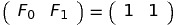
Multiplying this vector with the matrix M will get us to (F₁, F₂) = (1, 2):

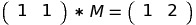
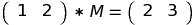
If we multiply (1, 2) with M, we get (F₂, F₃) = (2, 3):

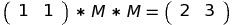
But we could get the same result by multiplying (1, 1) by M two times:

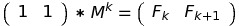
In general, multiplying k times by M gives us F_k, F_{k + 1}:

Here matrix exponentiation comes into play: multiplying k times by M is equal to multiplying by M^k:

Computing M^k takes O((size of M)³ * log(k)) time. In our problem, size of M is 2, so we can find N’th Fibonacci number in O(2³ * log(N)) = O(log(N)):

function fibonacci_exponentiation(N):
  if N <= 1:
    return 1
  initial = (1, 1)
  exp = matrix_power_with_modulo(M, N - 1, 1000000007) // assuming we’ve defined M
  return (initial * exp)[1][2] modulo 1000000007

We multiply our initial vector (1, 1) by M^{N - 1} and get initial * exp = (F_{N - 1}, F_N). We must return F_N, so we take it from first row, second column of initial * exp. All indexation is done starting from 1.

Finding N’th element of linear recurrent sequence

Let’s take a look at more general problem than before. Sequence A satisfies two properties:

1. A_i = c₁ * A_{i - 1} + c₂ * A_{i - 2} + … + c_k * A_{i - k} for i ≥ k (c₁, c₂ …, c_k are given integers);
2. A₀ = a₀, A₁ = a₁, …, A_{k - 1} = a_{k - 1} (a₀, a₁, …, a_{k - 1} are given integers).
   We need to find A_N modulo 1000000007, when N is up to 10¹⁸ and k up to 50.

Side note: such a sequence A_i is called recurrent, because computing A_i requires computing A_j for some j < i. Also, A_i is called linear, because it depends linearly on A_j for some j < i.

Notice that if we take k = 2, a₀ = a₁ = 1, c₁ = c₂ = 1, then this sequence will be Fibonacci sequence from the previous problem.

Here we will look for a solution that involves matrix multiplication right from the start. If we obtain matrix M, such that:

then we can get A_N in the following manner:

Two questions arise:

1. What is the number of rows and columns of M?
   The reasoning is the same as with Fibonacci numbers: we multiply matrix with 1 row and k columns by M, and get matrix with 1 row and k columns.
   Therefore, M has k rows and k columns. In other words, M is square matrix with size k;
2. What are the values in M? Let’s denote them as x_ij:
   
   Then we can write down equations, which are based on the definition of matrix multiplication:
   
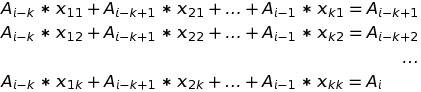
   From the first equation it is easy to see, that x₂₁ = 1 and x_i1 = 0 for i = 1, 3, 4, …, k.
   From the second equation we conclude that x₃₂ = 1 and x_i2 = 0 for i = 1, 2, 4, …, k.
   Following this logic up to k-1’th equation, we get x_i,i-1 = 1 for i = 2, 3, …, k and x_ij = 0 for i = 1, 2, 3, …, k and j ≤ k - 1, j ≠ i - 1.
   The last equation looks like the definition of A_i. Based on that, we get x_ik = c_{k - i +1}:
   

Now, when we have M, there are no more obstacles. We can implement the solution.
Pseudo code:

function recurrent_seq(N, k, a, c): // a and c are arrays of size k
  if N <= k - 1:
    return a[N]
  M = build_M(k, c)
  initial = a // initial vector: (a_0, a_1, …, a_{k-1})
  exp = matrix_power_with_modulo(M, N - k + 1, 1000000007)
  return (initial * exp)[1][k] modulo 1000000007 // initial*exp is a matrix (A_{N - k + 1}, A_{N - k + 2}, …, A_N). We take first row, last column as the result, which is A_N.

This code will run in O(k³ * log(N)) if we use fast matrix exponentiation.

Finding the sum of Fibonacci numbers up to N

Let’s go back to Fibonacci numbers:

1. F₀ = F₁ = 1;
2. F_i = F_{i - 1} + F_{i - 2} for i ≥ 2.

Introduce a new sequence: P_i = F₀ + F₁ + … + F_i (i.e. sum of first i Fibonacci numbers).
The problem is: find P_N modulo 1000000007 for N up to 10¹⁸.

Surprisingly, we can do it with matrices again. Let’s imagine we have a matrix M, such that:

Then we can obtain P_N by doing:

By now you must be familiar with the method of obtaining M and determining its size. I’ll present you M right away:

The first column is three 1’s, because P_i = P_{i - 1} + F_i = P_{i - 1} + F_{i - 2} + F_{i - 1}.

You can find sum of first N numbers of any recurrent linear sequence A_i, not just Fibonacci. To do that, introduce the “sum sequence” P_i = A₀ + A₁ + … + A_i. Put this sequence into the initial vector. Then find the matrix that gives you P_{i + 1}, based on P_i and some A’s.

Computing multiple linear recurrent sequences at once

Take a look at the problem Candy Distribution 3 from HackerEarth Medium Track. Basically, it asks, given integer n ≥ 10⁶, find the number of pairs of integers (x, y) such that:

1. 0 ≤ x < 2ⁿ;
2. 0 ≤ y < 2ⁿ;
3. Bitwise OR of x and y is not equal to x;
4. Bitwise OR of x and y is not equal to y.

When solving this problem, I came up with the following solution: let dp_i be the answer for n = i. Then it can be shown that:
dp_i = dp_{i - 1} * 4 + g_{i - 1} * 2 for i > 1,
dp₁ = 0,
where sequence g satisfies:
g_i = g_{i - 1} * 3 + 2^{i - 1} for i > 1,
g₁ = 1.

Side note: this is not the only way to solve this problem. For example, there is another approach proposed in the editorial. Also, due to this specific problem constraints’ (namely, up to 10⁶ inputs for each test), it can not be accepted with matrix exponentiation.

There are 3 recurrent sequences involved: dp_i depends on g_{i - 1}, g_i depends on 2^{i - 1} (powers of two can be viewed as recurrent sequence P_i: P₀ = 1, P_i = 2 * P_{i - 1}). What if we want to compute dp_n using matrix exponentiation?

Find a matrix M, such that:

One can see that:

How to come up with M without much thinking?
Notice, that in the first column we have 4, 2 and 0. This is precisely because
dp_i = dp_{i - 1} * 4 + g_{i - 1} * 2 + 2^{i - 1} * 0
Generally, if the value at row i and column j equals x, then i’th column of initial vector has the coefficient x when calculating j’th column of resulting vector. For example, value in first row and third column is 0, because 2ⁱ = 0 * dp_{i - 1} + … .

The answer for this problem would be the first row and first column of

Solving dynamic programming problems with fixed linear transitions

Let’s take a look at another HackerEarth problem: PK and interesting language. It goes like this:

Count the number of strings of length L with lowercase english letters, if some pairs of letters can not appear consequently in those strings. L is up to 10⁷, there are up to 100 inputs.

The “banned” pairs are described in the input as matrix: banned[i][j] == 0 means that letter j can not go after letter i in a valid string. Otherwise, banned[i][j] == 1.

Let dp[n][last_letter] be the number of valid strings of length n, which have last letter equal to last_letter. Then we can recalculate dp in order of increasing n:

dp[1][a] = dp[1][b] = … = dp[1][z] = 1
for n = 2..L:
  for last_letter = a..z:
    for next_letter = a..z:
      if banned[last_letter][next_letter] != 0:
        dp[n + 1][next_letter] += dp[n][last_letter]

The logic behind this is such: if we have the number of valid strings for some n and last_letter (it is dp[n][last_letter]), then we can add some letter to the end of those strings. Let’s iterate over this new letter next_letter and see if it is OK to place it after last_letter. If it is, then adding next_letter will result in the string of length n + 1 with last letter equal to next_letter. Thus, we add dp[n][last_letter] to dp[n + 1][next_letter].

The above approach works in Θ(L * 26²) time and won’t pass with L ~ 10⁷.

To speed things up, notice that inside the
for n = 2..L
loop nothing depends on n itself! Well, you could argue that writing “dp[n + 1][next_letter] += dp[n][last_letter]” and then saying “it does not depend on n” is nonsense. What I want to stress out is that transition from n to n + 1 happens in exactly the same way like, for example, from n + 100 to n + 101. The “banned” rules do not change over time!

The second observation would be: transition formulas from n to n + 1 are linear. To compute dp[n + 1][next_letter], we sum up dp[n][letter] for some letter. We do not have something like
dp[n + 1][next_letter] += dp[n][letter] * dp[n][next_letter],
which would mean that transition is not linear.

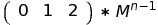
These two observations combined provide a useful property: there exists some matrix M, such that for any n ≥ 1

By now you should be able to tell that M is a square matrix with size 26 (which is number of letters in English alphabet). It contains 26 * 26 = 676 values - tough thing if you want to write them down manually!
Here is the easy way to understand, which values x_ij must be in M, based on the above equation:

1. Call the left part initial and the right part result;
2. By matrix multiplication definition we have:
   
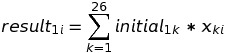
3. In other words, when you want to compute i-th value of the result, you take all x’s from i-th column and multiply them by corresponding initial’s;
4. This means that x_ki is the number, which tells “how many times we need to add initial_1k to result_1i”. Personally, I call it “impact of k-th value on i-th value of dp”.

In this problem, M is conveniently given to you in input. Indeed, we could rewrite the transition loop to this:

for last_letter = a..z:
  for next_letter = a..z:
    dp[n + 1][next_letter] += dp[n][last_letter] * banned[last_letter][next_letter]

That’s because “banned” is given in binary form: 1 if letters can appear together, 0 in other case.
The states of dynamic programming here are letters, and matrix “banned” shows how one letter affect the other. The final solution is:

It works in O(26³ * log(L)), which is significantly faster and passes time limit.

This way of speeding up dynamic programming is crucial to understand. Most of the problems tagged “Matrix exponentiation” on HackerEarth can be solved with this trick.

Implementation

Generally, you’d want to express three functions in your code:

1. Multiply two matrices of appropriate sizes;
2. Create an identity matrix I_n;
3. Raise a matrix to r-th power using fast exponentiation. Also you should consider a way to store your matrix.

The most straight-forward approach is to store matrices as 2D-arrays:

int matrix_1[50][50];
int matrix_2[50][50];

While the easiest way to perform multiplication is to use hard-coded operands:

int mat_a[50][50], mat_b[50][50];

void mul()
{
  // multiplies mat_a by mat_b
}

For example, it could look like this:

const int MAX_SIZE = 50;
const int MOD = 1e9 + 7;

int a[MAX_SIZE][MAX_SIZE];
int b[MAX_SIZE][MAX_SIZE];
int tmp[MAX_SIZE][MAX_SIZE];

void mul_mat(int n1, int m1, int n2, int m2)
{   
    // Instead of passing the matrices, we pass only their dimensions.
    // Function multiplies a by b if 
    //   a has n1 rows and m1 columns
    //   b has n2 rows and m2 columns
    // The result is stored in tmp matrix, then copied to a.
    //
    // Notice that the resulting matrix has n1 rows and m2 columns.

    memset(tmp, 0, sizeof(tmp));
    assert(m1 == n2); // according to definition of matrix multiplication

    for(int i = 0; i < n1; i++)
        for(int j = 0; j < m2; j++) {
            for(int k = 0; k < m1; k++) {
                tmp[i][j] = (tmp[i][j] + a[i][k] * 1ll * b[k][j]) % MOD;
            }
        }

    memcpy(a, tmp, sizeof(a));
}

void create_identity(int n)
{   
    // Creates identity matrix I_n and stores it in a.
    for(int i = 0; i < n; i++)
        for(int j = 0; j < n; j++)
            if(i == j)
                a[i][j] = 1;
            else
                a[i][j] = 0;
}

The exponentiating function is tricky to write in such case. So, if I have enough time, I prefer to implement Matrix as a class in C++:

const int MOD = 1e9 + 7;

struct Matrix
{
    vector< vector<int> > mat; // the contents of matrix as a 2D-vector
    int n_rows, n_cols; // number of rows and columns

    Matrix(vector< vector<int> > values): mat(values), n_rows(values.size()),
        n_cols(values[0].size()) {}

    static Matrix identity_matrix(int n)
    {
        // Return I_n - the identity matrix of size n.
        // This function is static, because it creates a new Matrix instance
        vector< vector<int> > values(n, vector<int>(n, 0));
        for(int i = 0; i < n; i++)
            values[i][i] = 1;
        return values;
    }

    Matrix operator*(const Matrix &other) const 
    {
        int n = n_rows, m = other.n_cols;
        vector< vector<int> > result(n_rows, vector<int>(m, 0));
        for(int i = 0; i < n; i++)
            for(int j = 0; j < m; j++) {
                for(int k = 0; k < n_cols; k++) {
                    result[i][j] = (result[i][j] + mat[i][k] * 1ll * other.mat[k][j]) % MOD;
                }
            }
        // Multiply matrices as usual, then return the result as the new Matrix
        return Matrix(result);
    }

    inline bool is_square() const
    {
        return n_rows == n_cols;
    }
};

Matrix fast_exponentiation(Matrix m, int power)
{
    assert(m.is_square());
    Matrix result = Matrix::identity_matrix(m.n_rows);

    while(power) {
        if(power & 1)
            result = result * m;
        m = m * m;
        power >>= 1;
    }

    return result;
}

Remember, this implementation is only meant for learning purposes. You may come up with better (faster, more readable, more C++-ish) approach.

There are two tricks I want to mention, that speed up usual computations:

1. If the modulo MOD in problem is such, that MOD² fits into long long, then you can reduce number of modulo operations to O(n²) (in case of multiplying two n x n matrices A and B).
2. If you problem requires answering many queries of raising the same matrix M to some power, you can precalculate powers of two of M to get things done faster. My solution for Candy Distribution 3 using this trick (and some others):

const int MOD = 1e9 + 7;
const long long MOD2 = static_cast<long long>(MOD) * MOD;
const int MAX_K = 50;

struct Matrix
{
    vector< vector<int> > mat;
    int n_rows, n_cols;

    Matrix() {}

    Matrix(vector< vector<int> > values): mat(values), n_rows(values.size()),
        n_cols(values[0].size()) {}

    static Matrix identity_matrix(int n)
    {
        vector< vector<int> > values(n, vector<int>(n, 0));
        for(int i = 0; i < n; i++)
            values[i][i] = 1;
        return values;
    }

    Matrix operator*(const Matrix &other) const 
    {
        int n = n_rows, m = other.n_cols;
        vector< vector<int> > result(n_rows, vector<int>(n_cols, 0));
        for(int i = 0; i < n; i++)
            for(int j = 0; j < m; j++) {
                long long tmp = 0;
                for(int k = 0; k < n_cols; k++) {
                    tmp += mat[i][k] * 1ll * other.mat[k][j];
                    while(tmp >= MOD2)
                        tmp -= MOD2;
                }
                result[i][j] = tmp % MOD;
            }

        return move(Matrix(move(result)));
    }

    inline bool is_square() const
    {
        return n_rows == n_cols;
    }
};

// M_powers[i] is M, raised to 2^i-th power
Matrix M_powers[55];

void precalc_powers(Matrix M)
{
    assert(M.is_square());
    M_powers[0] = M;

    for(int i = 1; i < 55; i++)
        M_powers[i] = M_powers[i - 1] * M_powers[i - 1];
}

Matrix fast_exponentiation_with_precalc(int power)
{
    Matrix result = Matrix::identity_matrix(M_powers[0].mat.size());
    int pointer = 0;
    while(power) {
        if(power & 1)
            result = result * M_powers[pointer];
        pointer++;
        power >>= 1;
    }
    return result;
}

inline int get_int()
{
    char c;
    int ret = 0;
    while(isdigit(c = getchar()))
        ret = ret * 10 + c - '0';
    return ret;
}

int main()
{
    int t;
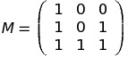
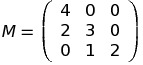
    Matrix M({ 
            {4, 0, 0}, 
            {2, 3, 0}, 
            {0, 1, 2} });
    precalc_powers(M);

    Matrix initial({ {0, 1, 2} });
    t = get_int();
    for(int i = 0; i < t; i++) {
        int n = get_int();
        cout << (initial * fast_exponentiation_with_precalc(n - 1)).mat[0][0] << "\n";
    }
}

(however, it can not pass all tests, because the intended solution is pure precalculation).

The modulo trick alone:

long long MOD2 = MOD * MOD;
for(int i = 0; i < n; i++)
  for(int j = 0; j < n; j++) {
    long long tmp = 0;
    for(int k = 0; k < n; k++) {
      // Since A and B are taken modulo MOD, the product A[i][k] * B[k][j] is
      // not more than MOD * MOD.
      tmp += A[i][k] * 1ll * B[k][j];
      while(tmp >= MOD2) // Taking modulo MOD2 is easy, because we can do it by subtraction
       tmp -= MOD2;
      }
    result[i][j] = tmp % MOD; // One % operation per resulting element
  }

In general, solutions using matrix multiplication are very short. The longest code I’ve written was 201 lines, and it was really tedious problem.

Practice problems

There are many beautiful problems on HackerEarth, that benefit from matrix exponentiation. My first encounter with this technique started with the problem “Tiles” from December Clash.

Most problems here require a dynamic programming solution, which is later improved by fast exponentiation.

1. PK and interesting language
   Difficulty: easy
   Comment: problem is explained in this article, so you should be able to implement it right away.
2. Tiles
   Difficulty: medium-hard
   Prerequisites: bitmask dynamic programming
   Comment: surprisingly, this problem does not have tag “Matrix exponentiation”.
3. ABCD strings
   Difficulty: medium-hard
   Comment: harder version of “PK and interesting language”. Here you have to come up with the matrix yourself. Mine was of size 16.
4. Mehta and the difficult task, Mehta and the evil strings
   Difficulty: medium
   Prerequisites: basics of bitmasking
   Comment: two similar problems from the same author. Once you solve either of them, the other one should be easy.
5. Long walks from office to home sweet home
   Difficulty: easy-medium
   Comment: somewhat similar to “PK and interesting language”.