In graph theory, a flow network is defined as a directed graph involving a source($$S$$) and a sink($$T$$) and several other nodes connected with edges. Each edge has an individual capacity which is the maximum limit of flow that edge could allow.
Flow in the network should follow the following conditions:
- For any non-source and non-sink node, the input flow is equal to output flow.
- For any edge($$E_i$$) in the network, $$ 0 \le flow(E_i) \le Capacity(E_i) $$.
- Total flow out of the source node is equal total to flow in to the sink node.
- Net flow in the edges follows skew symmetry i.e. $$F(u,v) = -F(v,u)$$ where $$F(u,v)$$ is flow from node u to node v. This leads to a conclusion where you have to sum up all the flows between two nodes(either directions) to find net flow between the nodes initially.
Maximum Flow:
It is defined as the maximum amount of flow that the network would allow to flow from source to sink. Multiple algorithms exist in solving the maximum flow problem. Two major algorithms to solve these kind of problems are Ford-Fulkerson algorithm and Dinic's Algorithm. They are explained below.
Ford-Fulkerson Algorithm:
It was developed by L. R. Ford, Jr. and D. R. Fulkerson in 1956. A pseudocode for this algorithm is given below,
Inputs required are network graph $$G$$, source node $$S$$ and sink node $$T$$.
function: FordFulkerson(Graph G,Node S,Node T):
    Initialise flow in all edges to 0
    while (there exists an augmenting path(P) between S and T in residual network graph):
        Augment flow between S to T along the path P
        Update residual network graph
    return
An augmenting path is a simple path from source to sink which do not include any cycles and that pass only through positive weighted edges. A residual network graph indicates how much more flow is allowed in each edge in the network graph. If there are no augmenting paths possible from $$S$$ to $$T$$, then the flow is maximum. The result i.e. the maximum flow will be the total flow out of source node which is also equal to total flow in to the sink node.
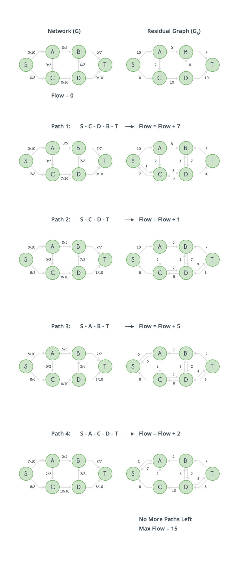
A demonstration of working of Ford-Fulkerson algorithm is shown below with the help of diagrams.
Implementation:
- An augmenting path in residual graph can be found using DFS or BFS.
- Updating residual graph includes following steps: (refer the diagrams for better understanding)
- For every edge in the augmenting path, a value of minimum capacity in the path is subtracted from all the edges of that path.
- An edge of equal amount is added to edges in reverse direction for every successive nodes in the augmenting path.
The complexity of Ford-Fulkerson algorithm cannot be accurately computed as it all depends on the path from source to sink. For example, considering the network shown below, if each time, the path chosen are $$S-A-B-T$$ and $$S-B-A-T$$ alternatively, then it can take a very long time. Instead, if path chosen are only $$S-A-T$$ and $$S-B-T$$, would also generate the maximum flow.

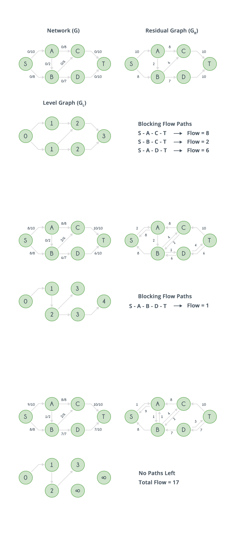
Dinic's Algorithm
In 1970, Y. A. Dinitz developed a faster algorithm for calculating maximum flow over the networks. It includes construction of level graphs and residual graphs and finding of augmenting paths along with blocking flow.
Level graph is one where value of each node is its shortest distance from source.
Blocking flow includes finding the new path from the bottleneck node.
Residual graph and augmenting paths are previously discussed.
Pseudocode for Dinic's algorithm is given below.
Inputs required are network graph G, source node S and sink node T.
function: DinicMaxFlow(Graph G,Node S,Node T):
    Initialize flow in all edges to 0, F = 0
    Construct level graph
    while (there exists an augmenting path in level graph):
        find blocking flow f in level graph
        F = F + f
        Update level graph
    return F
Update of level graph includes removal of edges with full capacity. Removal of nodes that are not sink and are dead ends. A demonstration of working of Dinic's algorithm is shown below with the help of diagrams.