
If this is the first time you hear about graphs, I strongly recommend to first read a great introduction to graph theory which has been prepared by Prateek. It contains all necessary definitions for this text. In this tutorial I will be talking about shortest paths in a Graph. Graphs can represent a lot of real-life networks like a state highway network, a network of cities or any other collections of objects that can be modeled as a network. The shortest path algorithm becomes very useful in finding out the least resource intensive path from one node of the network to the other.
Shortest Paths
We will start with one of the most studied and very interesting problem in graph theory - finding shortest paths between vertices. This problem is defined for graphs which have lengths associated with its edges.
But first things first, we need a few basic definitions to begin with.
A path in a graph is a sequence of vertices in which every two consecutive vertices are connected. If the first vertex of the paths is v and the last is u, we say that the path is a path from v to u.
Most of the time, we are interested in paths which do not have repeated vertices. These paths are called simple paths.
Since we want to find shortest paths, we have to define what a length of a path is. This is simple and straightforward, the length of a path is the sum of lengths of its edges.
Now we are ready to start examining the problem. Actually, we can create a distinction between the two major versions of it:
-
Single Source Shortest Paths (SSSP): for a source vertex s, we want to find the shortest paths from s to all other vertices in the graph.
-
All Pairs Shortest Paths (APSP): for every pair of vertices (u, v), we are interested in finding the shortest paths between them.
From now, we will focus on finding the lengths of the shortest paths. However, all methods presented here can be extended to find the exact paths.
Of course, if we are able to solve SSSP, we are also able to solve APSP by solving SSSP problem for every vertex as the source vertex. While this method is absolutely correct, as we will see, it is not always optimal.
First, let's start with SSSP (Single Source Shortest Paths) problem.
Notice that if a graph has uniform length of all edges, you should be already able to solve it (for sure if you are familiar with Graph Monk I). Actually this is very simple, because if all edges have the same length, then the shortest path between two vertices is a path which has the fewer number of edges from all such paths and we already know that it can be solved with Breadth First Search (BFS) .
The problem becomes harder if lengths are not uniform. The shortest path can have many more edges that any other path. Consider the following example (lengths are presented near the edges):
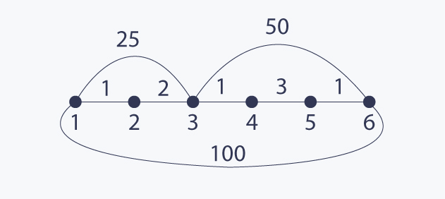
The shortest path between 1 and 6 has length 8 and contains 5 edges, while any other path from 1 to 6 has fewer edges and is longer. It is easy to see that BFS does not work here.
Now we know something about the nature of the problem, so let's start solving it. Probably the most famous algorithm for solving it is the Dijsktra algorithm. It is based on a crucial assumption that all edges have non negative weights. Its correct logic strongly depends on this assumption - the algorithm does not work if the graph has negative edges.
Let d(s, v) be the length of shortest path from source vertex s to vertex v. It is super easy to think about the state of execution of this algorithm as of partition the set V of all vertices into two disjoint sets X := {v : such that d(s, v) has its final value already computed} and V X. Initially V X is empty and we initialize d(s, s) := 0 and d(s, v) := infinity for all v != s.
Then as long as V X in not empty i.e there is at least one vertex v for which d(s, v) in not already computed, we repeat the following step:
Let v be a vertex in V X such that d(s, v) is minimal from all such vertices.
We move v to X and for each edge (v, u) such that v is in V X, we update the current distance to u, i.e we do d(s, u) = min(d(s, u), d(s, v) + w(v, u)), where w(v, u) is the length of the edge from v to u.
And that is all! The most important thing here is the following invariant:
As long as V / X in not empty, there exists v in V X such that d(s, v) has already assigned its final value. This is true because we are dealing only with non negative edges here and this vertex has to have the minimal value of d(s, v) from all vertices in V X from the same fact. I encourage all of you to prove that this invariant is fulfilled in every step of the execution of the algorithm - it is a great exercise!
What is the time complexity of Dijkstra algorithm? Well, let's examine that. We have n iterations of the main loop here, because in each iteration we move one vertex to the set X. In each iteration, we select a vertex v which has the minimum value of d(s, v) from vertices in V X. Then we update distance values for all neighbours of v. It is easy to see that during the execution, we select this minimum exactly n times and we update distance values exactly m times, because we do it once for every edge. Let f(n) be the time complexity of selecting our minimum and let g(n) be the time complexity of the update operation. Then the total complexity is O(n * f(n) + m * g(n)). We can implement both these functions in many different ways. Probably the most common implementation is to use a heap based priority queue with decrease-key operation for updating distance values or to use use a balanced binary tree. Both these methods gives time complexity O(n logn + m logn). There are many cases that we can do better than that, for example, if length are small integers or if we can use more advanced priority queues like fibonacci heap. But these methods are rather too complicated for this text, nevertheless it is worth to know that they exists.
Finally, let's see what may happen in we have negative length edges. Let's consider the following graph:
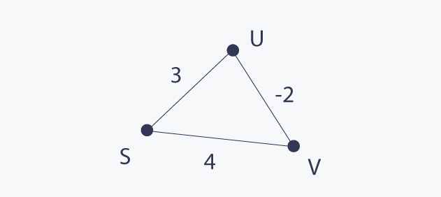
Dijkstra algorithm will not work here, because it will assign d(s, s) := 0, then d(s, u) := 3 and finally d(s, v) := 1, but actually there exists a path from s to u of length 2.
So what we do when we have to deal with negative lengths of edges? We definitely have to use a different method and Bellman-Ford (BF) algorithm is a great one.
The idea behind this algorithm is to have computed shortests paths which uses at most k edges in the k-th iteration of the algorithm. After n - 1 iterations, all shortest paths are computed, because a simple path in a graph with n vertices can have at most n - 1 edges.
for v in V:
    if v == s:
        d[v] := 0
    else:
        d[v] := INFINITY

for i = 1 to n - 1:
    for (u, v) in E:
        d[v] := min(d[v], d[u] + length(u, v))
In order to see why the algorithm is correct, we can notice that if u, ..., w, v is the shortest path from u to v, then it can be constructed from the shortest path from u to w by adding the edge between w and v to it. This is a very important and widely used fact about shortest paths - remember it.
A nice thing about Bellman-Ford is the fact that it works for negative edges also. The only assumption here is that the input graph cannot contain a negative length cycle, because the problem is not well defined in such graphs (you can construct a path of arbitrary small length). Actually, this algorithm can be used to detect if a graph contains a negative length cycle.
The time complexity of Bellman-Ford is O(n * m), because we do n iterations and in each of them, we examine all edges in the graph. While the algorithm was invented a long time ago, it is still the fastest strongly polynomial i.e. its polynomial complexity depends only on the number of vertices and the number of edges, method to find shortest paths in general graphs with arbitrary edges lengths.
APSP (All pairs shortest paths)
In this version of the problem, we need to find the shortest paths between all pairs of vertices. The most straightforward method to do that is to use any known algorithm for SSSP version of the problem and run it from every vertex as a source. This results in O(n * m log n) time if we use Dijkstra and O(n^2 * m) if we use Bellman-Ford. This is nice if we do not have to deal deal with negative edges, because Dijksta is quite fast then, although we will take a look at the algorithm which runs in O(n^3) even if there are negative length edges. This algorithm is called Floyd-Warshall (FW) and it is a great application of dynamic programming.
The algorithm is based on the following idea:
Let d(i, j, k) be the shortest path between i and j which uses only vertices with numbers in {1, 2, ..., k}. Then d(i, j, n) is the desired result which we want to compute for all i and j. Let's assume that we have computed d(i, j, k) for all i and j, and we want to compute d(i, j, k + 1) now. There are two cases to consider. The shortest path between i and j which uses vertices in {1, 2, ..., k + 1} may either use the vertex with number k+1 or not. If it does not use it, then it is equal to d(i, j, k). If it uses vertex k+1, it is equal d(i, k + 1, k) + d(k + 1, j, k), because of the fact given in description of Bellman-Ford algorithm and due to the fact that the vertex k+1 can occur only once in such a path.
for v in V:
    for u in V:
        if v == u:
            d[v][u] := 0
        else:
            d[v][u] := INFINITY

for (u, v) in E:
    d[u][v] := length(u, v)

for k = 1 to n:
    for i = 1 to n:
        for j = 1 to n:
            d[i][j] = min(d[i][j], d[i][k] + d[k][j])
This algorithm is a great example of dynamic programming which you probably noticed. Its running time is O(n^3), because we do n iterations and in each of them we examine all pairs of vertices. In fact, it can be implemented to use only O(n^2) space and the paths itselves can also be reconstructed very fast.
DAG
DAG (directed acyclic graph) is a directed graph which does not contain directed cycles
![[PICTURE 3]](https://he-s3.s3.amazonaws.com/media/uploads/c91c9dd.jpg)
While it looks very simple, it is widely used to solve many problems. Probably the most interesting fact about DAGs is that its vertices can be sorted in such a way that if v is before u in this sorted order, then there is no edge from u to v, i.e. if we examine vertices in sorted order from left to right, all edges are directed from left to right also. This order is called topological order. You can notice that there can be more that one topological sorting of vertices for a given graph.
Are you interested to know how to sort vertices of a DAG in topological order?
It is easy to see that the first vertex can be any vertex which does not use any incoming edges and it must exist at least one such vertex, because DAGs do not have directed cycles. If we pick any such vertex, put it in the resulting order, and delete it from the graph, the resulting graph will remain a DAG and we can continue this process while the graph has at least one vertex.
This is probably the most intuitive method for computing a topological order, but while it can be implemented to run in O(n + m) time, it may not be the easiest one to implement.
If you want a more clever way to do that, and definitely easier to implement, you can use DFS for that.
Let exit[v] be the time during DFS in which we fully processed the subtree rooted in v in resulted DFS tree:
cur_time := 0
dfs(v):
    visited[v] := true
    for u in adj[v]:
        if not visited[u]:
            dfs(u)
    exit[v] := cur_time
    cur_time += 1
Then vertices printed in decreasing order of exit times produce a valid topological order. This is true, because there can be no edge from a vertex with smaller exit time to a vertex with greater one, because it will imply that there is a directed cycle in the graph.
Author
{"5901655": "/users/pagelets/trending_card/?sensual=True"}