
Introduction
For freshers, projects are the best way to highlight their data science knowledge. In fact, not just freshers, up to mid-level experienced professionals can keep their resumes updated with new, interesting projects. After all, they don't come easy. It takes a lot of time to create a project which can truly showcase the depth and breadth of your knowledge.
I hope this project will help you gain much needed knowledge and help your resume get shortlisted faster. This project shows all the steps (from scratch) taken to solve a Machine Learning problem. For your understanding, I've taken a simple yet challenging data set where you can engineer features at your discretion as well.
We'll participate in a Kaggle competition and make our way up the leaderboard among ~ top 14% participants.
This project is most suitable for people who have a basic understanding of python and Machine Learning. Even if you are absolutely new to it, give it a try. And ask questions in Comments below. R users can refer to this equivalent R script and follow the explanation given below.
Table of Contents
- Process of Machine Learning Predictions
- Housing Data Set
- Understand the problem
- Hypothesis Generation
- Get Data
- Data Exploration
- Data Pre-Processing
- Feature Engineering - Create 331 new features
- Model Training - XGBoost, Neural Network, Lasso
- Model Evaluation
Process of Machine Learning Predictions
“Keep tormenting data until it starts revealing its hidden secrets.” Yes, it can be done but there's a way around it. Making predictions using Machine Learning isn't just about grabbing the data and feeding it to algorithms. The algorithm might spit out some prediction but that's not what you are aiming for. The difference between good data science professionals and naive data science aspirants is that the former set follows this process religiously. The process is as follows: 1. Understand the problem: Before getting the data, we need to understand the problem we are trying to solve. If you know the domain, think of which factors could play an epic role in solving the problem. If you don't know the domain, read about it. 2. Hypothesis Generation: This is quite important, yet it is often forgotten. In simple words, hypothesis generation refers to creating a set of features which could influence the target variable given a confidence interval ( taken as 95% all the time). We can do this before looking at the data to avoid biased thoughts. This step often helps in creating new features. 3. Get Data: Now, we download the data and look at it. Determine which features are available and which aren't, how many features we generated in hypothesis generation hit the mark, and which ones could be created. Answering these questions will set us on the right track. 4. Data Exploration: We can't determine everything by just looking at the data. We need to dig deeper. This step helps us understand the nature of variables (skewed, missing, zero variance feature) so that they can be treated properly. It involves creating charts, graphs (univariate and bivariate analysis), and cross-tables to understand the behavior of features. 5. *Data Preprocessing: *Here, we impute missing values and clean string variables (remove space, irregular tabs, data time format) and anything that shouldn't be there. This step is usually followed along with the data exploration stage. 6. Feature Engineering: Now, we create and add new features to the data set. Most of the ideas for these features come during the hypothesis generation stage. 7. Model Training: Using a suitable algorithm, we train the model on the given data set. 8. Model Evaluation: Once the model is trained, we evaluate the model's performance using a suitable error metric. Here, we also look for variable importance, i.e., which variables have proved to be significant in determining the target variable. And, accordingly we can shortlist the best variables and train the model again. 9. Model Testing: Finally, we test the model on the unseen data (test data) set.
We'll follow this process in the project to arrive at our final predictions. Let's get started.
1.Understand the problem
The data set for this project has been taken from Kaggle's Housing Data Set Knowledge Competition. As mentioned above, the data set is simple. This project aims at predicting house prices (residential) in Ames, Iowa, USA. I believe this problem statement is quite self-explanatory and doesn't need more explanation. Hence, we move to the next step.
2. Hypothesis Generation
Well, this is going to be interesting. What factors can you think of right now which can influence house prices ? As you read this, I want you to write down your factors as well, then we can match them with the data set. Defining a hypothesis has two parts: Null Hypothesis (Ho) and Alternate Hypothesis(Ha). They can be understood as:
Ho - There exists no impact of a particular feature on the dependent variable. Ha - There exists a direct impact of a particular feature on the dependent variable.
Based on a decision criterion (say, 5% significance level), we always 'reject' or 'fail to reject' the null hypothesis in statistical parlance. Practically, while model building we look for probability (p) values. If p value < 0.05, we reject the null hypothesis. If p > 0.05, we fail to reject the null hypothesis. Some factors which I can think of that directly influence house prices are the following:
- Area of House
- How old is the house
- Location of the house
- How close/far is the market
- Connectivity of house location with transport
- How many floors does the house have
- What material is used in the construction
- Water /Electricity availability
- Play area / parks for kids (if any)
- If terrace is available
- If car parking is available
- If security is available
…keep thinking. I am sure you can come up with many more apart from these.
3. Get Data
You can download the data and load it in your python IDE. Also, check the competition page where all the details about the data and variables are given. The data set consists of 81 explanatory variables. Yes, it's going to be one heck of a data exploration ride. But, we'll learn how to deal with so many variables. The target variable is SalePrice. As you can see the data set comprises numeric, categorical, and ordinal variables. Without further ado, let's start with hands-on coding.
4. Data Exploration
Data Exploration is the key to getting insights from data. Practitioners say a good data exploration strategy can solve even complicated problems in a few hours. A good data exploration strategy comprises the following:
- Univariate Analysis - It is used to visualize one variable in one plot. Examples: histogram, density plot, etc.
- Bivariate Analysis - It is used to visualize two variables (x and y axis) in one plot. Examples: bar chart, line chart, area chart, etc.
- Multivariate Analysis - As the name suggests, it is used to visualize more than two variables at once. Examples: stacked bar chart, dodged bar chart, etc.
- Cross Tables -They are used to compare the behavior of two categorical variables (used in pivot tables as well).
Let's load the necessary libraries and data and start coding.
#Loading libraries
import numpy as np
import pandas as pd
import matplotlib.pyplot as plt
%matplotlib inline
plt.rcParams['figure.figsize'] = (10.0, 8.0)
import seaborn as sns
from scipy import stats
from scipy.stats import norm
#loading data
train = pd.read_csv("/data/Housing/train.csv")
test = pd.read_csv("/data/Housing/test.csv")
train.head()
| Id | MSSubClass | MSZoning | LotFrontage | LotArea | Street | Alley | LotShape | LandContour | Utilities | ... | PoolArea | PoolQC | Fence | MiscFeature | MiscVal | MoSold | YrSold | SaleType | SaleCondition | |
|---|---|---|---|---|---|---|---|---|---|---|---|---|---|---|---|---|---|---|---|---|
| 0 | 1 | 60 | RL | 65.0 | 8450 | Pave | NaN | Reg | Lvl | AllPub | ... | 0 | NaN | NaN | NaN | 0 | 2 | 2008 | WD | Normal |
| 1 | 2 | 20 | RL | 80.0 | 9600 | Pave | NaN | Reg | Lvl | AllPub | ... | 0 | NaN | NaN | NaN | 0 | 5 | 2007 | WD | Normal |
| 2 | 3 | 60 | RL | 68.0 | 11250 | Pave | NaN | IR1 | Lvl | AllPub | ... | 0 | NaN | NaN | NaN | 0 | 9 | 2008 | WD | Normal |
| 3 | 4 | 70 | RL | 60.0 | 9550 | Pave | NaN | IR1 | Lvl | AllPub | ... | 0 | NaN | NaN | NaN | 0 | 2 | 2006 | WD | Abnorml |
| 4 | 5 | 60 | RL | 84.0 | 14260 | Pave | NaN | IR1 | Lvl | AllPub | ... | 0 | NaN | NaN | NaN | 0 | 12 | 2008 | WD | Normal |
print ('The train data has {0} rows and {1} columns'.format(train.shape[0],train.shape[1]))
print ('----------------------------')
print ('The test data has {0} rows and {1} columns'.format(test.shape[0],test.shape[1]))
The train data has 1460 rows and 81 columns
----------------------------
The test data has 1459 rows and 80 columns
Alternatively, you can also check the data set information using the info() command.
train.info()
Let's check if the data set has any missing values.
#check missing values
train.columns[train.isnull().any()]

['LotFrontage',
 'Alley',
 'MasVnrType',
 'MasVnrArea',
 'BsmtQual',
 'BsmtCond',
 'BsmtExposure',
 'BsmtFinType1',
 'BsmtFinType2',
 'Electrical',
 'FireplaceQu',
 'GarageType',
 'GarageYrBlt',
 'GarageFinish',
 'GarageQual',
 'GarageCond',
 'PoolQC',
 'Fence',
 'MiscFeature']
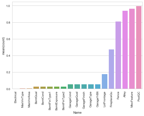
Out of 81 features, 19 features have missing values. Let's check the percentage of missing values in these columns.
#missing value counts in each of these columns
miss = train.isnull().sum()/len(train)
miss = miss[miss > 0]
miss.sort_values(inplace=True)
miss
| Electrical | 0.000685 |
| MasVnrType | 0.005479 |
| MasVnrArea | 0.005479 |
| BsmtQual | 0.025342 |
| BsmtCond | 0.025342 |
| BsmtFinType1 | 0.025342 |
| BsmtExposure | 0.026027 |
| BsmtFinType2 | 0.026027 |
| GarageCond | 0.055479 |
| GarageQual | 0.055479 |
| GarageFinish | 0.055479 |
| GarageType | 0.055479 |
| GarageYrBlt | 0.055479 |
| LotFrontage | 0.177397 |
| FireplaceQu | 0.472603 |
| Fence | 0.807534 |
| Alley | 0.937671 |
| MiscFeature | 0.963014 |
| PoolQC | 0.995205 |
| dtype: float64 |
We can infer that the variable PoolQC has 99.5% missing values followed by MiscFeature, Alley, and Fence. Let's look at a pretty picture explaining these missing values using a bar plot.
#visualising missing values
miss = miss.to_frame()
miss.columns = ['count']
miss.index.names = ['Name']
miss['Name'] = miss.index

#plot the missing value count
sns.set(style="whitegrid", color_codes=True)
sns.barplot(x = 'Name', y = 'count', data=miss)
plt.xticks(rotation = 90)
sns.plt.show()
Let's proceed and check the distribution of the target variable.
#SalePrice
sns.distplot(train['SalePrice'])
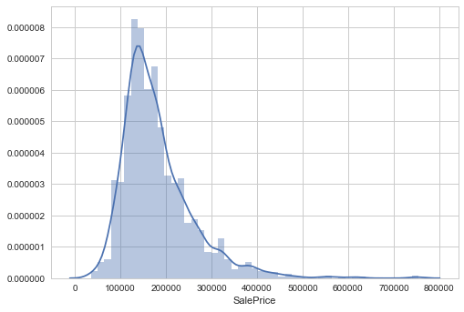
We see that the target variable SalePrice has a right-skewed distribution. We'll need to log transform this variable so that it becomes normally distributed. A normally distributed (or close to normal) target variable helps in better modeling the relationship between target and independent variables. In addition, linear algorithms assume constant variance in the error term. Alternatively, we can also confirm this skewed behavior using the skewness metric.
#skewness
print "The skewness of SalePrice is {}".format(train['SalePrice'].skew())
The skewness of SalePrice is 1.88287575977
#now transforming the target variable
target = np.log(train['SalePrice'])
print ('Skewness is', target.skew())
sns.distplot(target)
Skewness is 0.12133506220520406)
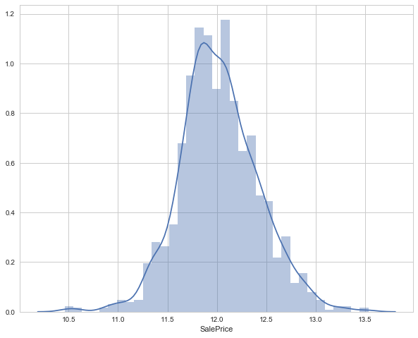
As you saw, log transformation of the target variable has helped us fixing its skewed distribution and the new distribution looks closer to normal. Since we have 80 variables, visualizing one by one wouldn't be an astute approach. Instead, we'll look at some variables based on their correlation with the target variable. However, there's a way to plot all variables at once, and we'll look at it as well. Moving forward, we'll separate numeric and categorical variables and explore this data from a different angle.
#separate variables into new data frames
numeric_data = train.select_dtypes(include=[np.number])
cat_data = train.select_dtypes(exclude=[np.number])
print ("There are {} numeric and {} categorical columns in train data".format(numeric_data.shape[1],cat_data.shape[1]))`
del numeric_data['Id']
Now, we are interested to learn about the correlation behavior of numeric variables. Out of 38 variables, I presume some of them must be correlated. If found, we can later remove these correlated variables as they won't provide any useful information to the model.
#correlation plot
corr = numeric_data.corr()
sns.heatmap(corr)
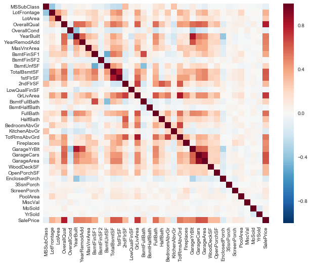
Notice the last row of this map. We can see the correlation of all variables against SalePrice. As you can see, some variables seem to be strongly correlated with the target variable. Here, a numeric correlation score will help us understand the graph better.
print (corr['SalePrice'].sort_values(ascending=False)[:15], '\n') #top 15 values
print ('----------------------')
print (corr['SalePrice'].sort_values(ascending=False)[-5:]) #last 5 values`

SalePrice       1.000000
OverallQual     0.790982
GrLivArea       0.708624
GarageCars      0.640409
GarageArea      0.623431
TotalBsmtSF     0.613581
1stFlrSF        0.605852
FullBath        0.560664
TotRmsAbvGrd    0.533723
YearBuilt       0.522897
YearRemodAdd    0.507101
GarageYrBlt     0.486362
MasVnrArea      0.477493
Fireplaces      0.466929
BsmtFinSF1      0.386420
Name: SalePrice, dtype: float64, '\n')
----------------------
YrSold          -0.028923
OverallCond     -0.077856
MSSubClass      -0.084284
EnclosedPorch   -0.128578
KitchenAbvGr    -0.135907
Name: SalePrice, dtype: float64</pre>
OverallQual feature is 79% correlated with the target variable. Overallqual feature refers to the overall material and quality of the materials of the completed house. Well, this make sense as well. People usually consider these parameters for their dream house. In addition, GrLivArea is 70% correlated with the target variable. GrLivArea refers to the living area (in sq ft.) above ground. The following variables show people also care about if the house has a garage, the area of that garage, the size of the basement area, etc.
Let's check the OverallQual variable in detail.
train['OverallQual'].unique()
array([ 7,  6,  8,  5,  9,  4, 10,  3,  1,  2])
The overall quality is measured on a scale of 1 to 10. Hence, we can fairly treat it as an ordinal variable. An ordinal variable has an inherent order. For example, Rank of students in class, data collected on Likert scale, etc. Let's check the median sale price of houses with respect to OverallQual. You might be wondering, “Why median ?” We are using median because the target variable is skewed. A skewed variable has outliers and median is robust to outliers.
We can create such aggregated tables using pandas pivot tables quite easily.
#let's check the mean price per quality and plot it.
pivot = train.pivot_table(index='OverallQual', values='SalePrice', aggfunc=np.median)
pivot.sort
| 1 | 50150 |
| 2 | 60000 |
| 3 | 86250 |
| 4 | 108000 |
| 5 | 133000 |
| 6 | 160000 |
| 7 | 200141 |
| 8 | 269750 |
| 9 | 345000 |
| 10 | 432390 |
| Name: SalePrice, dtype: int64 |
Let's plot this table and understand the median behavior using a bar graph.
pivot.plot(kind='bar', color='red')
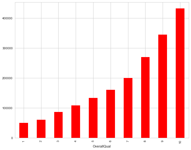
This behavior is quite normal. As the overall quality of a house increases, its sale price also increases. Let's visualize the next correlated variable GrLivArea and understand their behavior.
#GrLivArea variable
sns.jointplot(x=train['GrLivArea'], y=train['SalePrice'])
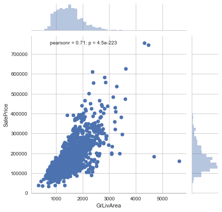
As seen above, here also we see a direct correlation of living area with sale price. However, we can spot an outlier value GrLivArea > 5000. I've seen outliers play a significant role in spoiling a model's performance. Hence, we'll get rid of it. If you are enjoying this activity, you can visualize other correlated variables as well. Now, we'll move forward and explore categorical features. The simplest way to understand categorical variables is using .describe() command.
cat_data.describe()
| MSZoning | Street | Alley | LotShape | LandContour | Utilities | LotConfig | LandSlope | Neighborhood | Condition1 | ... | GarageType | GarageFinish | GarageQual | GarageCond | PavedDrive | PoolQC | Fence | MiscFeature | SaleType | SaleCondition | |
|---|---|---|---|---|---|---|---|---|---|---|---|---|---|---|---|---|---|---|---|---|---|
| count | 1460 | 1460 | 91 | 1460 | 1460 | 1460 | 1460 | 1460 | 1460 | 1460 | ... | 1379 | 1379 | 1379 | 1379 | 1460 | 7 | 281 | 54 | 1460 | |
| unique | 5 | 2 | 2 | 4 | 4 | 2 | 5 | 3 | 25 | 9 | ... | 6 | 3 | 5 | 5 | 3 | 3 | 4 | 4 | 9 | 6 |
| top | RL | Pave | Grvl | Reg | Lvl | AllPub | Inside | Gtl | NAmes | Norm | ... | Attchd | Unf | TA | TA | Y | Gd | MnPrv | Shed | WD | Normal |
| freq | 1151 | 1454 | 50 | 925 | 1311 | 1459 | 1052 | 1382 | 225 | 1260 | ... | 870 | 605 | 1311 | 1326 | 1340 | 3 | 157 | 49 | 1267 | 1198 |
Let's check the median sale price of a house based on its SaleCondition. SaleCondition explains the condition of sale. Not much information is given about its categories.
sp_pivot = train.pivot_table(index='SaleCondition', values='SalePrice', aggfunc=np.median)
sp_pivot
| SaleCondition | |
| Abnorml | 130000 |
| AdjLand | 104000 |
| Alloca | 148145 |
| Family | 140500 |
| Normal | 160000 |
| Partial | 244600 |
| Name: SalePrice, dtype: int64 |
sp_pivot.plot(kind='bar',color='red')
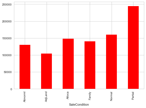
We see that SaleCondition Partial has the highest mean sale price. Though, due to lack of information we can't generate many insights from this data. Moving forward, like we used correlation to determine the influence of numeric features on SalePrice. Similarly, we'll use the ANOVA test to understand the correlation between categorical variables and SalePrice. ANOVA test is a statistical technique used to determine if there exists a significant difference in the mean of groups. For example, let's say we have two variables A and B. Each of these variables has 3 levels (a1,a2,a3 and b1,b2,b3). If the mean of these levels with respect to the target variable is the same, the ANOVA test will capture this behavior and we can safely remove them.
While using ANOVA, our hypothesis is as follows:
Ho - There exists no significant difference between the groups. Ha - There exists a significant difference between the groups.
Now, we'll define a function which calculates p values. From those p values, we'll calculate a disparity score. Higher the disparity score, better the feature in predicting sale price.
cat = [f for f in train.columns if train.dtypes[f] == 'object']
def anova(frame):
    anv = pd.DataFrame()
    anv['features'] = cat
    pvals = []
    for c in cat:
           samples = []
           for cls in frame[c].unique():
                  s = frame[frame[c] == cls]['SalePrice'].values
                  samples.append(s)
           pval = stats.f_oneway(*samples)[1]
           pvals.append(pval)
    anv['pval'] = pvals
    return anv.sort_values('pval')

cat_data['SalePrice'] = train.SalePrice.values
k = anova(cat_data)
k['disparity'] = np.log(1./k['pval'].values)
sns.barplot(data=k, x = 'features', y='disparity')
plt.xticks(rotation=90)
plt

Here we see that among all categorical variablesNeighborhoodturned out to be the most important feature followed by ExterQual, KitchenQual, etc. It means that people also consider the goodness of the neighborhood, the quality of the kitchen, the quality of the material used on the exterior walls, etc. Finally, to get a quick glimpse of all variables in a data set, let's plot histograms for all numeric variables to determine if all variables are skewed. For categorical variables, we'll create a boxplot and understand their nature.
#create numeric plots
num = [f for f in train.columns if train.dtypes[f] != 'object']
num.remove('Id')
nd = pd.melt(train, value_vars = num)
n1 = sns.FacetGrid (nd, col='variable', col_wrap=4, sharex=False, sharey = False)
n1 = n1.map(sns.distplot, 'value')
n1

As you can see, most of the variables are right skewed. We'll have to transform them in the next stage. Now, let's create boxplots for visualizing categorical variables.
def boxplot(x,y,**kwargs):
            sns.boxplot(x=x,y=y)
            x = plt.xticks(rotation=90)

cat = [f for f in train.columns if train.dtypes[f] == 'object']

p = pd.melt(train, id_vars='SalePrice', value_vars=cat)
g = sns.FacetGrid (p, col='variable', col_wrap=2, sharex=False, sharey=False, size=5)
g = g.map(boxplot, 'value','SalePrice')
g

Here, we can see that most of the variables possess outlier values. It would take us days if we start treating these outlier values one by one. Hence, for now we'll leave them as is and let our algorithm deal with them. As we know, tree-based algorithms are usually robust to outliers.
5. Data Pre-Processing
In this stage, we'll deal with outlier values, encode variables, impute missing values, and take every possible initiative which can remove inconsistencies from the data set. If you remember, we discovered that the variable GrLivArea has outlier values. Precisely, one point crossed the 4000 mark. Let's remove that:
#removing outliers
train.drop(train[train['GrLivArea'] > 4000].index, inplace=True)
train.shape #removed 4 rows`
(1456, 81)
In row 666, in the test data, it was found that information in variables related to 'Garage' (GarageQual, GarageCond, GarageFinish, GarageYrBlt) is missing. Let's impute them using the mode of these respective variables.
#imputing using mode
test.loc[666, 'GarageQual'] = "TA" #stats.mode(test['GarageQual']).mode
test.loc[666, 'GarageCond'] = "TA" #stats.mode(test['GarageCond']).mode
test.loc[666, 'GarageFinish'] = "Unf" #stats.mode(test['GarageFinish']).mode
test.loc[666, 'GarageYrBlt'] = "1980" #np.nanmedian(test['GarageYrBlt'])`
In row 1116, in test data, all garage variables are NA except GarageType. Let's mark it NA as well.
#mark as missing
test.loc[1116, 'GarageType'] = np.nan
Now, we'll encode all the categorical variables. This is necessary because most ML algorithms do not accept categorical values, instead they are expected to be converted to numerical. LabelEncoder function from sklearn is used to encode variables. Let's write a function to do this:
#importing function
from sklearn.preprocessing import LabelEncoder
le = LabelEncoder()
def factorize(data, var, fill_na = None):
      if fill_na is not None:
            data[var].fillna(fill_na, inplace=True)
      le.fit(data[var])
      data[var] = le.transform(data[var])
      return data
LotFrontage variable using the median value of LotFrontage by Neighborhood. Such imputation strategies are built during data exploration. I suggest you spend some more time on data exploration. To do this, we should combine our train and test data so that we can modify both the data sets at once. Also, it'll save our time.
#combine the data set
alldata = train.append(test)
alldata.shape
(2915, 81)
The combined data set has 2915 rows and 81 columns. Now, we'll impute the LotFrontage variable.
#impute lotfrontage by median of neighborhood
lot_frontage_by_neighborhood = train['LotFrontage'].groupby(train['Neighborhood'])

for key, group in lot_frontage_by_neighborhood:
                idx = (alldata['Neighborhood'] == key) & (alldata['LotFrontage'].isnull())
                alldata.loc[idx, 'LotFrontage'] = group.median()
#imputing missing values
alldata["MasVnrArea"].fillna(0, inplace=True)
alldata["BsmtFinSF1"].fillna(0, inplace=True)
alldata["BsmtFinSF2"].fillna(0, inplace=True)
alldata["BsmtUnfSF"].fillna(0, inplace=True)
alldata["TotalBsmtSF"].fillna(0, inplace=True)
alldata["GarageArea"].fillna(0, inplace=True)
alldata["BsmtFullBath"].fillna(0, inplace=True)
alldata["BsmtHalfBath"].fillna(0, inplace=True)
alldata["GarageCars"].fillna(0, inplace=True)
alldata["GarageYrBlt"].fillna(0.0, inplace=True)
alldata["PoolArea"].fillna(0, inplace=True)
qual_dict = {np.nan: 0, "Po": 1, "Fa": 2, "TA": 3, "Gd": 4, "Ex": 5}
name = np.array(['ExterQual','PoolQC' ,'ExterCond','BsmtQual','BsmtCond','HeatingQC','KitchenQual','FireplaceQu', 'GarageQual','GarageCond'])

for i in name:
     alldata[i] = alldata[i].map(qual_dict).astype(int)

alldata["BsmtExposure"] = alldata["BsmtExposure"].map({np.nan: 0, "No": 1, "Mn": 2, "Av": 3, "Gd": 4}).astype(int)

bsmt_fin_dict = {np.nan: 0, "Unf": 1, "LwQ": 2, "Rec": 3, "BLQ": 4, "ALQ": 5, "GLQ": 6}
alldata["BsmtFinType1"] = alldata["BsmtFinType1"].map(bsmt_fin_dict).astype(int)
alldata["BsmtFinType2"] = alldata["BsmtFinType2"].map(bsmt_fin_dict).astype(int)
alldata["Functional"] = alldata["Functional"].map({np.nan: 0, "Sal": 1, "Sev": 2, "Maj2": 3, "Maj1": 4, "Mod": 5, "Min2": 6, "Min1": 7, "Typ": 8}).astype(int)

alldata["GarageFinish"] = alldata["GarageFinish"].map({np.nan: 0, "Unf": 1, "RFn": 2, "Fin": 3}).astype(int)
alldata["Fence"] = alldata["Fence"].map({np.nan: 0, "MnWw": 1, "GdWo": 2, "MnPrv": 3, "GdPrv": 4}).astype(int)

#encoding data
alldata["CentralAir"] = (alldata["CentralAir"] == "Y") * 1.0
varst = np.array(['MSSubClass','LotConfig','Neighborhood','Condition1','BldgType','HouseStyle','RoofStyle','Foundation','SaleCondition'])

for x in varst:
         factorize(alldata, x)

#encode variables and impute missing values
alldata = factorize(alldata, "MSZoning", "RL")
alldata = factorize(alldata, "Exterior1st", "Other")
alldata = factorize(alldata, "Exterior2nd", "Other")
alldata = factorize(alldata, "MasVnrType", "None")
alldata = factorize(alldata, "SaleType", "Oth")`
6. Feature Engineering
There are no libraries or sets of functions you can use to engineer features. Well, there are some but not as effective. It's majorly a manual task but believe me, it's fun. Feature engineering requires domain knowledge and lots of creative ideas. The ideas for new features usually develop during the data exploration and hypothesis generation stages. The motive of feature engineering is to create new features which can help make predictions better.
As you can also see, there's a massive scope of feature engineering in this data set. Now let's create new features from the given list of 81 features. Make sure you follow this section carefully.
Most categorical variables have near-zero variance distribution. Near-zero variance distribution is when one of the categories in a variable has >90% of the values. We'll create some binary variables depicting the presence or absence of a category. The new features will contain 0 or 1 values. In addition, we'll create some more variables which are self-explanatory with comments.
#creating new variable (1 or 0) based on irregular count levels
#The level with highest count is kept as 1 and rest as 0
alldata["IsRegularLotShape"] = (alldata["LotShape"] == "Reg") * 1
alldata["IsLandLevel"] = (alldata["LandContour"] == "Lvl") * 1
alldata["IsLandSlopeGentle"] = (alldata["LandSlope"] == "Gtl") * 1
alldata["IsElectricalSBrkr"] = (alldata["Electrical"] == "SBrkr") * 1
alldata["IsGarageDetached"] = (alldata["GarageType"] == "Detchd") * 1
alldata["IsPavedDrive"] = (alldata["PavedDrive"] == "Y") * 1
alldata["HasShed"] = (alldata["MiscFeature"] == "Shed") * 1
alldata["Remodeled"] = (alldata["YearRemodAdd"] != alldata["YearBuilt"]) * 1

#Did the modeling happen during the sale year?
alldata["RecentRemodel"] = (alldata["YearRemodAdd"] == alldata["YrSold"]) * 1

# Was this house sold in the year it was built?
alldata["VeryNewHouse"] = (alldata["YearBuilt"] == alldata["YrSold"]) * 1
alldata["Has2ndFloor"] = (alldata["2ndFlrSF"] == 0) * 1
alldata["HasMasVnr"] = (alldata["MasVnrArea"] == 0) * 1
alldata["HasWoodDeck"] = (alldata["WoodDeckSF"] == 0) * 1
alldata["HasOpenPorch"] = (alldata["OpenPorchSF"] == 0) * 1
alldata["HasEnclosedPorch"] = (alldata["EnclosedPorch"] == 0) * 1
alldata["Has3SsnPorch"] = (alldata["3SsnPorch"] == 0) * 1
alldata["HasScreenPorch"] = (alldata["ScreenPorch"] == 0) * 1

#setting levels with high count as 1 and the rest as 0
#you can check for them using the value_counts function
alldata["HighSeason"] = alldata["MoSold"].replace(` `{1: 0, 2: 0, 3: 0, 4: 1, 5: 1, 6: 1, 7: 1, 8: 0, 9: 0, 10: 0, 11: 0, 12: 0})
alldata["NewerDwelling"] = alldata["MSSubClass"].replace(` `{20: 1, 30: 0, 40: 0, 45: 0,50: 0, 60: 1, 70: 0, 75: 0, 80: 0, 85: 0,` `90: 0, 120: 1, 150: 0, 160: 0, 180: 0, 190: 0})
alldata.shape
(2915, 100)
Now, we have 100 features in the data. It means we create 19 more columns. Let's continue and create some more features. Once again, we'll combine the original train and test files to create a parallel alldata2 file. This file will have original feature values. We'll use this data as reference to create more features.
#create alldata2
alldata2 = train.append(test)

alldata["SaleCondition_PriceDown"] = alldata2.SaleCondition.replace({'Abnorml': 1, 'Alloca': 1, 'AdjLand': 1, 'Family': 1, 'Normal': 0, 'Partial': 0})

# house completed before sale or not
alldata["BoughtOffPlan"] = alldata2.SaleCondition.replace({"Abnorml" : 0, "Alloca" : 0, "AdjLand" : 0, "Family" : 0, "Normal" : 0, "Partial" : 1})
alldata["BadHeating"] = alldata2.HeatingQC.replace({'Ex': 0, 'Gd': 0, 'TA': 0, 'Fa': 1, 'Po': 1})
#calculating total area using all area columns
area_cols = ['LotFrontage', 'LotArea', 'MasVnrArea', 'BsmtFinSF1', 'BsmtFinSF2', 'BsmtUnfSF',` `'TotalBsmtSF', '1stFlrSF', '2ndFlrSF', 'GrLivArea', 'GarageArea', 'WoodDeckSF',` `'OpenPorchSF', 'EnclosedPorch', '3SsnPorch', 'ScreenPorch', 'LowQualFinSF', 'PoolArea' ]

alldata["TotalArea"] = alldata[area_cols].sum(axis=1)
alldata["TotalArea1st2nd"] = alldata["1stFlrSF"] + alldata["2ndFlrSF"]
alldata["Age"] = 2010 - alldata["YearBuilt"]
alldata["TimeSinceSold"] = 2010 - alldata["YrSold"]
alldata["SeasonSold"] = alldata["MoSold"].map({12:0, 1:0, 2:0, 3:1, 4:1, 5:1, 6:2, 7:2, 8:2, 9:3, 10:3, 11:3}).astype(int)
alldata["YearsSinceRemodel"] = alldata["YrSold"] - alldata["YearRemodAdd"]

# Simplifications of existing features into bad/average/good based on counts
alldata["SimplOverallQual"] = alldata.OverallQual.replace({1 : 1, 2 : 1, 3 : 1, 4 : 2, 5 : 2, 6 : 2, 7 : 3, 8 : 3, 9 : 3, 10 : 3})
alldata["SimplOverallCond"] = alldata.OverallCond.replace({1 : 1, 2 : 1, 3 : 1, 4 : 2, 5 : 2, 6 : 2, 7 : 3, 8 : 3, 9 : 3, 10 : 3})
alldata["SimplPoolQC"] = alldata.PoolQC.replace({1 : 1, 2 : 1, 3 : 2, 4 : 2})
alldata["SimplGarageCond"] = alldata.GarageCond.replace({1 : 1, 2 : 1, 3 : 1, 4 : 2, 5 : 2})
alldata["SimplGarageQual"] = alldata.GarageQual.replace({1 : 1, 2 : 1, 3 : 1, 4 : 2, 5 : 2})
alldata["SimplFireplaceQu"] = alldata.FireplaceQu.replace({1 : 1, 2 : 1, 3 : 1, 4 : 2, 5 : 2})
alldata["SimplFireplaceQu"] = alldata.FireplaceQu.replace({1 : 1, 2 : 1, 3 : 1, 4 : 2, 5 : 2})
alldata["SimplFunctional"] = alldata.Functional.replace({1 : 1, 2 : 1, 3 : 2, 4 : 2, 5 : 3, 6 : 3, 7 : 3, 8 : 4})
alldata["SimplKitchenQual"] = alldata.KitchenQual.replace({1 : 1, 2 : 1, 3 : 1, 4 : 2, 5 : 2})
alldata["SimplHeatingQC"] = alldata.HeatingQC.replace({1 : 1, 2 : 1, 3 : 1, 4 : 2, 5 : 2})
alldata["SimplBsmtFinType1"] = alldata.BsmtFinType1.replace({1 : 1, 2 : 1, 3 : 1, 4 : 2, 5 : 2, 6 : 2})
alldata["SimplBsmtFinType2"] = alldata.BsmtFinType2.replace({1 : 1, 2 : 1, 3 : 1, 4 : 2, 5 : 2, 6 : 2})
alldata["SimplBsmtCond"] = alldata.BsmtCond.replace({1 : 1, 2 : 1, 3 : 1, 4 : 2, 5 : 2})
alldata["SimplBsmtQual"] = alldata.BsmtQual.replace({1 : 1, 2 : 1, 3 : 1, 4 : 2, 5 : 2})
alldata["SimplExterCond"] = alldata.ExterCond.replace({1 : 1, 2 : 1, 3 : 1, 4 : 2, 5 : 2})
alldata["SimplExterQual"] = alldata.ExterQual.replace({1 : 1, 2 : 1, 3 : 1, 4 : 2, 5 : 2})

#grouping neighborhood variable based on this plot
train['SalePrice'].groupby(train['Neighborhood']).median().sort_values().plot(kind='bar')
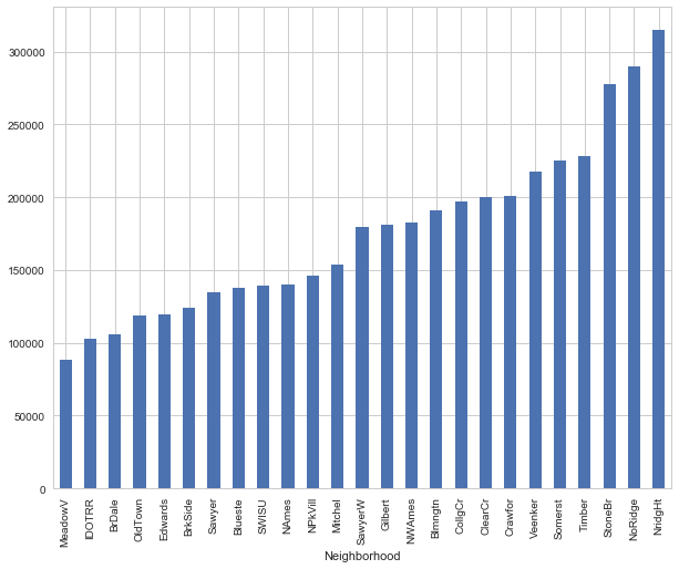
The graph above gives us a good hint on how to combine levels of the neighborhood variable into fewer levels. We can combine bars of somewhat equal height in one category. To do this, we'll simply create a dictionary and map it with variable values.
neighborhood_map = {"MeadowV" : 0, "IDOTRR" : 1, "BrDale" : 1, "OldTown" : 1, "Edwards" : 1, "BrkSide" : 1,` ` "Sawyer" : 1, "Blueste" : 1, "SWISU" : 2, "NAmes" : 2, "NPkVill" : 2, "Mitchel" : 2, "SawyerW" : 2, "Gilbert" : 2, "NWAmes" : 2, "Blmngtn" : 2, "CollgCr" : 2, "ClearCr" : 3, "Crawfor" : 3, "Veenker" : 3, "Somerst" : 3, "Timber" : 3, "StoneBr" : 4, "NoRidge" : 4, "NridgHt" : 4}

alldata['NeighborhoodBin'] = alldata2['Neighborhood'].map(neighborhood_map)
alldata.loc[alldata2.Neighborhood == 'NridgHt', "Neighborhood_Good"] = 1
alldata.loc[alldata2.Neighborhood == 'Crawfor', "Neighborhood_Good"] = 1
alldata.loc[alldata2.Neighborhood == 'StoneBr', "Neighborhood_Good"] = 1
alldata.loc[alldata2.Neighborhood == 'Somerst', "Neighborhood_Good"] = 1
alldata.loc[alldata2.Neighborhood == 'NoRidge', "Neighborhood_Good"] = 1
alldata["Neighborhood_Good"].fillna(0, inplace=True)
alldata["SaleCondition_PriceDown"] = alldata2.SaleCondition.replace({'Abnorml': 1, 'Alloca': 1, 'AdjLand': 1, 'Family': 1, 'Normal': 0, 'Partial': 0})

# House completed before sale or not
alldata["BoughtOffPlan"] = alldata2.SaleCondition.replace({"Abnorml" : 0, "Alloca" : 0, "AdjLand" : 0, "Family" : 0, "Normal" : 0, "Partial" : 1})
alldata["BadHeating"] = alldata2.HeatingQC.replace({'Ex': 0, 'Gd': 0, 'TA': 0, 'Fa': 1, 'Po': 1})
alldata.shape
(2915, 124)
Until this point, we've added 43 new features in the data set. Now, let's split the data into test and train and create some more features.
#create new data
train_new = alldata[alldata['SalePrice'].notnull()]
test_new = alldata[alldata['SalePrice'].isnull()]

print Train, train_new.shape
print ('----------------')
print Test, test_new.shape
Train (1456, 126)
----------------
Test (1459, 126)
Now, we'll transform numeric features and remove their skewness.
#get numeric features
numeric_features = [f for f in train_new.columns if train_new[f].dtype != object]

#transform the numeric features using log(x + 1)
from scipy.stats import skew
skewed = train_new[numeric_features].apply(lambda x: skew(x.dropna().astype(float)))
skewed = skewed[skewed > 0.75]
skewed = skewed.index
train_new[skewed] = np.log1p(train_new[skewed])
test_new[skewed] = np.log1p(test_new[skewed])
del test_new['SalePrice']
Now, we'll standardize the numeric features.
from sklearn.preprocessing import StandardScaler
scaler = StandardScaler()
scaler.fit(train_new[numeric_features])
scaled = scaler.transform(train_new[numeric_features])

for i, col in enumerate(numeric_features):
       train_new[col] = scaled[:,i]

numeric_features.remove('SalePrice')
scaled = scaler.fit_transform(test_new[numeric_features])

for i, col in enumerate(numeric_features):
      test_new[col] = scaled[:,i]
def onehot(onehot_df, df, column_name, fill_na):
       onehot_df[column_name] = df[column_name]
       if fill_na is not None:
            onehot_df[column_name].fillna(fill_na, inplace=True)

       dummies = pd.get_dummies(onehot_df[column_name], prefix="_"+column_name)
       onehot_df = onehot_df.join(dummies)
       onehot_df = onehot_df.drop([column_name], axis=1)
       return onehot_df

def munge_onehot(df):
       onehot_df = pd.DataFrame(index = df.index)

       onehot_df = onehot(onehot_df, df, "MSSubClass", None)
       onehot_df = onehot(onehot_df, df, "MSZoning", "RL")
       onehot_df = onehot(onehot_df, df, "LotConfig", None)
       onehot_df = onehot(onehot_df, df, "Neighborhood", None)
       onehot_df = onehot(onehot_df, df, "Condition1", None)
       onehot_df = onehot(onehot_df, df, "BldgType", None)
       onehot_df = onehot(onehot_df, df, "HouseStyle", None)
       onehot_df = onehot(onehot_df, df, "RoofStyle", None)
       onehot_df = onehot(onehot_df, df, "Exterior1st", "VinylSd")
       onehot_df = onehot(onehot_df, df, "Exterior2nd", "VinylSd")
       onehot_df = onehot(onehot_df, df, "Foundation", None)
       onehot_df = onehot(onehot_df, df, "SaleType", "WD")
       onehot_df = onehot(onehot_df, df, "SaleCondition", "Normal")

       #Fill in missing MasVnrType for rows that do have a MasVnrArea.
       temp_df = df[["MasVnrType", "MasVnrArea"]].copy()
       idx = (df["MasVnrArea"] != 0) & ((df["MasVnrType"] == "None") | (df["MasVnrType"].isnull()))
       temp_df.loc[idx, "MasVnrType"] = "BrkFace"
       onehot_df = onehot(onehot_df, temp_df, "MasVnrType", "None")

       onehot_df = onehot(onehot_df, df, "LotShape", None)
       onehot_df = onehot(onehot_df, df, "LandContour", None)
       onehot_df = onehot(onehot_df, df, "LandSlope", None)
       onehot_df = onehot(onehot_df, df, "Electrical", "SBrkr")
       onehot_df = onehot(onehot_df, df, "GarageType", "None")
       onehot_df = onehot(onehot_df, df, "PavedDrive", None)
       onehot_df = onehot(onehot_df, df, "MiscFeature", "None")
       onehot_df = onehot(onehot_df, df, "Street", None)
       onehot_df = onehot(onehot_df, df, "Alley", "None")
       onehot_df = onehot(onehot_df, df, "Condition2", None)
       onehot_df = onehot(onehot_df, df, "RoofMatl", None)
       onehot_df = onehot(onehot_df, df, "Heating", None)

       # we'll have these as numerical variables too
       onehot_df = onehot(onehot_df, df, "ExterQual", "None")
       onehot_df = onehot(onehot_df, df, "ExterCond", "None")
       onehot_df = onehot(onehot_df, df, "BsmtQual", "None")
       onehot_df = onehot(onehot_df, df, "BsmtCond", "None")
       onehot_df = onehot(onehot_df, df, "HeatingQC", "None")
       onehot_df = onehot(onehot_df, df, "KitchenQual", "TA")
       onehot_df = onehot(onehot_df, df, "FireplaceQu", "None")
       onehot_df = onehot(onehot_df, df, "GarageQual", "None")
       onehot_df = onehot(onehot_df, df, "GarageCond", "None")
       onehot_df = onehot(onehot_df, df, "PoolQC", "None")
       onehot_df = onehot(onehot_df, df, "BsmtExposure", "None")
       onehot_df = onehot(onehot_df, df, "BsmtFinType1", "None")
       onehot_df = onehot(onehot_df, df, "BsmtFinType2", "None")
       onehot_df = onehot(onehot_df, df, "Functional", "Typ")
       onehot_df = onehot(onehot_df, df, "GarageFinish", "None")
       onehot_df = onehot(onehot_df, df, "Fence", "None")
       onehot_df = onehot(onehot_df, df, "MoSold", None)

       # Divide  the years between 1871 and 2010 into slices of 20 years
       year_map = pd.concat(pd.Series("YearBin" + str(i+1), index=range(1871+i*20,1891+i*20))  for i in range(0, 7))
       yearbin_df = pd.DataFrame(index = df.index)
       yearbin_df["GarageYrBltBin"] = df.GarageYrBlt.map(year_map)
       yearbin_df["GarageYrBltBin"].fillna("NoGarage", inplace=True)
       yearbin_df["YearBuiltBin"] = df.YearBuilt.map(year_map)
       yearbin_df["YearRemodAddBin"] = df.YearRemodAdd.map(year_map)

       onehot_df = onehot(onehot_df, yearbin_df, "GarageYrBltBin", None)
       onehot_df = onehot(onehot_df, yearbin_df, "YearBuiltBin", None)
       onehot_df = onehot(onehot_df, yearbin_df, "YearRemodAddBin", None)
       return onehot_df

#create one-hot features
onehot_df = munge_onehot(train)

neighborhood_train = pd.DataFrame(index=train_new.shape)
neighborhood_train['NeighborhoodBin'] = train_new['NeighborhoodBin']
neighborhood_test = pd.DataFrame(index=test_new.shape)
neighborhood_test['NeighborhoodBin'] = test_new['NeighborhoodBin']

onehot_df = onehot(onehot_df, neighborhood_train, 'NeighborhoodBin', None)
train_new = train_new.join(onehot_df)
train_new.shape
(1456, 433)
Woah! This resulted in a whopping 433 columns. Similarly, we will add one-hot variables in test data as well.
#adding one hot features to test
onehot_df_te = munge_onehot(test)
onehot_df_te = onehot(onehot_df_te, neighborhood_test, "NeighborhoodBin", None)
test_new = test_new.join(onehot_df_te)
test_new.shape
(1459, 417)
The difference in number of train and test columns suggests that some new features in the train data aren't available in the test data. Let's remove those variables and keep an equal number of columns in the train and test data.
#dropping some columns from the train data as they are not found in test
drop_cols = ["_Exterior1st_ImStucc", "_Exterior1st_Stone","_Exterior2nd_Other","_HouseStyle_2.5Fin","_RoofMatl_Membran", "_RoofMatl_Metal", "_RoofMatl_Roll", "_Condition2_RRAe", "_Condition2_RRAn", "_Condition2_RRNn", "_Heating_Floor", "_Heating_OthW", "_Electrical_Mix", "_MiscFeature_TenC", "_GarageQual_Ex",  "_PoolQC_Fa"]
train_new.drop(drop_cols, axis=1, inplace=True)
train_new.shape
(1456, 417)
Now, we have an equal number of columns in the train and test data. Here, we'll remove a few more columns which either have lots of zeroes (hence doesn't provide any real information) or aren't available in either of the data sets.
#removing one column missing from train data
test_new.drop(["_MSSubClass_150"], axis=1, inplace=True)

# Drop these columns
drop_cols = ["_Condition2_PosN", # only two are not zero
         "_MSZoning_C (all)",
         "_MSSubClass_160"]

train_new.drop(drop_cols, axis=1, inplace=True)
test_new.drop(drop_cols, axis=1, inplace=True)
Let's transform the target variable and store it in a new array.
#create a label set
label_df = pd.DataFrame(index = train_new.index, columns = ['SalePrice'])
label_df['SalePrice'] = np.log(train['SalePrice'])
print("Training set size:", train_new.shape)
print("Test set size:", test_new.shape)

('Training set size:', (1456, 414))
('Test set size:', (1459, 413))
7. Model Training and Evaluation
Since our data is ready, we'll start training models now. We'll use three algorithms: XGBoost, Neural Network and Lasso Regression. Finally, we'll ensemble the models to generate final predictions.
import xgboost as xgb
regr = xgb.XGBRegressor(colsample_bytree=0.2,
                       gamma=0.0,
                       learning_rate=0.05,
                       max_depth=6,
                       min_child_weight=1.5,
                       n_estimators=7200,
                       reg_alpha=0.9,
                       reg_lambda=0.6,
                       subsample=0.2,
                       seed=42,
                       silent=1)

regr.fit(train_new, label_df)
from sklearn.metrics import mean_squared_error
def rmse(y_test,y_pred):
      return np.sqrt(mean_squared_error(y_test,y_pred))

# run prediction on training set to get an idea of how well it does
y_pred = regr.predict(train_new)
y_test = label_df
print("XGBoost score on training set: ", rmse(y_test, y_pred))
XGBoost score on training set: ', 0.037633322832013358)

# make prediction on test set
y_pred_xgb = regr.predict(test_new_one)

#submit this prediction and get the score
pred1 = pd.DataFrame({'Id': test['Id'], 'SalePrice': np.exp(y_pred_xgb)})
pred1.to_csv('xgbnono.csv', header=True, index=False)
from sklearn.linear_model import Lasso

#found this best alpha through cross-validation
best_alpha = 0.00099

regr = Lasso(alpha=best_alpha, max_iter=50000)
regr.fit(train_new, label_df)

# run prediction on the training set to get a rough idea of how well it does
y_pred = regr.predict(train_new)
y_test = label_df` `print("Lasso score on training set: ", rmse(y_test, y_pred))
<pre class="">('Lasso score on training set: ', 0.10175440647797629)</pre>
#make prediction on the test set
y_pred_lasso = regr.predict(test_new_one)
lasso_ex = np.exp(y_pred_lasso)
pred1 = pd.DataFrame({'Id': test['Id'], 'SalePrice': lasso_ex})
pred1.to_csv('lasso_model.csv', header=True, index=False)
Let's upload this file on Kaggle and check the score. We scored 0.11859 on the leaderboard. We see that the lasso model has outperformed the formidable XGBoost algorithm. And, it also improved our rank. With this, we have advanced into the top 16% of the participants. Since the data set is high dimensional (means large number of features), we can try our hands at building a neural network model as well. Let's do it. We'll use the keras library to train the neural network.
from keras.models import Sequential
from keras.layers import Dense
from keras.wrappers.scikit_learn import KerasRegressor
from sklearn.preprocessing import StandardScaler

np.random.seed(10)

#create Model
#define base model
def base_model():
     model = Sequential()
     model.add(Dense(20, input_dim=398, init='normal', activation='relu'))
     model.add(Dense(10, init='normal', activation='relu'))
     model.add(Dense(1, init='normal'))
     model.compile(loss='mean_squared_error', optimizer = 'adam')
     return model

seed = 7
np.random.seed(seed)

scale = StandardScaler()
X_train = scale.fit_transform(train_new)
X_test = scale.fit_transform(test_new)

keras_label = label_df.as_matrix()
clf = KerasRegressor(build_fn=base_model, nb_epoch=1000, batch_size=5,verbose=0)
clf.fit(X_train,keras_label)

#make predictions and create the submission file
kpred = clf.predict(X_test)
kpred = np.exp(kpred)
pred_df = pd.DataFrame(kpred, index=test["Id"], columns=["SalePrice"])
pred_df.to_csv('keras1.csv', header=True, index_label='Id')
#simple average
y_pred = (y_pred_xgb + y_pred_lasso) / 2
y_pred = np.exp(y_pred)
pred_df = pd.DataFrame(y_pred, index=test["Id"], columns=["SalePrice"])
pred_df.to_csv('ensemble1.csv', header=True, index_label='Id')
Summary
The project has been created to help people understand the complete process of machine learning / data science modeling. These steps ensure that you won't miss out any information in the data set and would also help another person understand your work. I would like to thank the Kaggle community for sharing info on competition forums which helped me a lot in creating this tutorial.
If you feel confident enough, you can register now for Machine Learning Challenge coming on May 30. It's going to be the biggest competitive machine learning event in India. I hope this tutorial helps you understand data science better. For any suggestions, concerns, and thoughts, feel free to write in Comments below.