
Introduction
Recruiters in the analytics/data science industry expect you to know at least two algorithms: Linear Regression and Logistic Regression. I believe you should have in-depth understanding of these algorithms. Let me tell you why.
Due to their ease of interpretation, consultancy firms use these algorithms extensively. Startups are also catching up fast. As a result, in an analytics interview, most of the questions come from linear and Logistic Regression.
In this article, you'll learn about Logistic Regression in detail. Believe me, Logistic Regression isn't easy to master. It does follow some assumptions like Linear Regression. But its method of calculating model fit and evaluation metrics is entirely different from Linear/Multiple regression.
But, don't worry! After you finish this tutorial, you'll become confident enough to explain Logistic Regression to your friends and even colleagues. Alongside theory, you'll also learn to implement Logistic Regression on a data set. I'll use R Language. In addition, we'll also look at various types of Logistic Regression methods.
Note: You should know basic algebra (elementary level). Also, if you are new to regression, I suggest you read how Linear Regression works first.
Table of Contents
- What is Logistic Regression ?
- What are the types of Logistic Regression techniques ?
- How does Logistic Regression work ?
- How can you evaluate Logistic Regression's model fit and accuracy ?
- Practical - Who survived on the Titanic ?
What is Logistic Regression ?
Many a time, situations arise where the dependent variable isn't normally distributed; i.e., the assumption of normality is violated. For example, think of a problem when the dependent variable is binary (Male/Female). Will you still use Multiple Regression? Of course not! Why? We'll look at it below.
Let's take a peek into the history of data analysis.
So, until 1972, people didn't know how to analyze data which has a non-normal error distribution in the dependent variable. Then, in 1972, came a breakthrough by John Nelder and Robert Wedderburn in the form of Generalized Linear Models. I'm sure you would be familiar with the term. Now, let's understand it in detail.
Generalized Linear Models are an extension of the linear model framework, which includes dependent variables which are non-normal also. In general, they possess three characteristics:
- These models comprise a linear combination of input features.
- The mean of the response variable is related to the linear combination of input features via a link function.
- The response variable is considered to have an underlying probability distribution belonging to the family of exponential distributions such as binomial distribution, Poisson distribution, or Gaussian distribution. Practically, binomial distribution is used when the response variable is binary. Poisson distribution is used when the response variable represents count. And, Gaussian distribution is used when the response variable is continuous.
Logistic Regression belongs to the family of generalized linear models. It is a binary classification algorithm used when the response variable is dichotomous (1 or 0). Inherently, it returns the set of probabilities of target class. But, we can also obtain response labels using a probability threshold value. Following are the assumptions made by Logistic Regression:
- The response variable must follow a binomial distribution.
- Logistic Regression assumes a linear relationship between the independent variables and the link function (logit).
- The dependent variable should have mutually exclusive and exhaustive categories.
In R, we use glm() function to apply Logistic Regression. In Python, we use sklearn.linear_model function to import and use Logistic Regression.
Note: We don't use Linear Regression for binary classification because its linear function results in probabilities outside [0,1] interval, thereby making them invalid predictions.
What are the types of Logistic Regression techniques ?
Logistic Regression isn't just limited to solving binary classification problems. To solve problems that have multiple classes, we can use extensions of Logistic Regression, which includes Multinomial Logistic Regression and Ordinal Logistic Regression. Let's get their basic idea:
1. Multinomial Logistic Regression: Let's say our target variable has K = 4 classes. This technique handles the multi-class problem by fitting K-1 independent binary logistic classifier model. For doing this, it randomly chooses one target class as the reference class and fits K-1 regression models that compare each of the remaining classes to the reference class.
Due to its restrictive nature, it isn't used widely because it does not scale very well in the presence of a large number of target classes. In addition, since it builds K - 1 models, we would require a much larger data set to achieve reasonable accuracy.
2. Ordinal Logistic Regression: This technique is used when the target variable is ordinal in nature. Let's say, we want to predict years of work experience (1,2,3,4,5, etc). So, there exists an order in the value, i.e., 5>4>3>2>1. Unlike a multinomial model, when we train K -1 models, Ordinal Logistic Regression builds a single model with multiple threshold values.
If we have K classes, the model will require K -1 threshold or cutoff points. Also, it makes an imperative assumption of proportional odds. The assumption says that on a logit (S shape) scale, all of the thresholds lie on a straight line.
Note: Logistic Regression is not a great choice to solve multi-class problems. But, it's good to be aware of its types. In this tutorial we'll focus on Logistic Regression for binary classification task.
How does Logistic Regression work?
Now comes the interesting part!
As we know, Logistic Regression assumes that the dependent (or response) variable follows a binomial distribution. Now, you may wonder, what is binomial distribution? Binomial distribution can be identified by the following characteristics:
- There must be a fixed number of trials denoted by n, i.e. in the data set, there must be a fixed number of rows.
- Each trial can have only two outcomes; i.e., the response variable can have only two unique categories.
- The outcome of each trial must be independent of each other; i.e., the unique levels of the response variable must be independent of each other.
- The probability of success (p) and failure (q) should be the same for each trial.
Let's understand how Logistic Regression works. For Linear Regression, where the output is a linear combination of input feature(s), we write the equation as:
`Y = βo + β1X + ∈`
In Logistic Regression, we use the same equation but with some modifications made to Y. Let's reiterate a fact about Logistic Regression: we calculate probabilities. And, probabilities always lie between 0 and 1. In other words, we can say:
- The response value must be positive.
- It should be lower than 1.
First, we'll meet the above two criteria. We know the exponential of any value is always a positive number. And, any number divided by number + 1 will always be lower than 1. Let's implement these two findings:
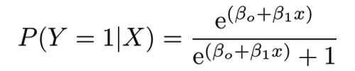
This is the logistic function.
Now we are convinced that the probability value will always lie between 0 and 1. To determine the link function, follow the algebraic calculations carefully. P(Y=1|X) can be read as "probability that Y =1 given some value for x." Y can take only two values, 1 or 0. For ease of calculation, let's rewrite P(Y=1|X) as p(X).
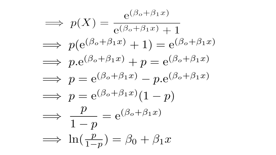
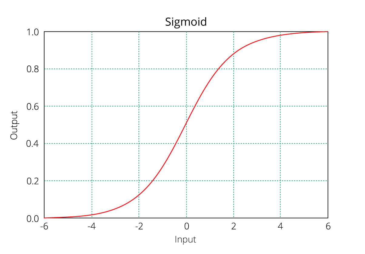
As you might recognize, the right side of the (immediate) equation above depicts the linear combination of independent variables. The left side is known as the log - odds or odds ratio or logit function and is the link function for Logistic Regression. This link function follows a sigmoid (shown below) function which limits its range of probabilities between 0 and 1.
 Until here, I hope you've understood how we derive the equation of Logistic Regression. But how is it interpreted?
We can interpret the above equation as, a unit increase in variable x results in multiplying the odds ratio by ε to power β. In other words, the regression coefficients explain the change in log(odds) in the response for a unit change in predictor. However, since the relationship between p(X) and X is not straight line, a unit change in input feature doesn't really affect the model output directly but it affects the odds ratio.
This is contradictory to Linear Regression where, regardless of the value of input feature, the regression coefficient always represents a fixed increase/decrease in the model output per unit increase in the input feature.
In Multiple Regression, we use the Ordinary Least Square (OLS) method to determine the best coefficients to attain good model fit. In Logistic Regression, we use maximum likelihood method to determine the best coefficients and eventually a good model fit.
Maximum likelihood works like this: It tries to find the value of coefficients (βo,β1) such that the predicted probabilities are as close to the observed probabilities as possible. In other words, for a binary classification (1/0), maximum likelihood will try to find values of βo and β1 such that the resultant probabilities are closest to either 1 or 0. The likelihood function is written as

How can you evaluate Logistic Regression model fit and accuracy ?
In Linear Regression, we check adjusted R², F Statistics, MAE, and RMSE to evaluate model fit and accuracy. But, Logistic Regression employs all different sets of metrics. Here, we deal with probabilities and categorical values. Following are the evaluation metrics used for Logistic Regression:
1. Akaike Information Criteria (AIC)
You can look at AIC as counterpart of adjusted r square in multiple regression. It's an important indicator of model fit. It follows the rule: Smaller the better. AIC penalizes increasing number of coefficients in the model. In other words, adding more variables to the model wouldn't let AIC increase. It helps to avoid overfitting.
Looking at the AIC metric of one model wouldn't really help. It is more useful in comparing models (model selection). So, build 2 or 3 Logistic Regression models and compare their AIC. The model with the lowest AIC will be relatively better.
2. Null Deviance and Residual Deviance
Deviance of an observation is computed as -2 times log likelihood of that observation. The importance of deviance can be further understood using its types: Null and Residual Deviance. Null deviance is calculated from the model with no features, i.e.,only intercept. The null model predicts class via a constant probability.
Residual deviance is calculated from the model having all the features.On comarison with Linear Regression, think of residual deviance as residual sum of square (RSS) and null deviance as total sum of squares (TSS). The larger the difference between null and residual deviance, better the model.
Also, you can use these metrics to compared multiple models: whichever model has a lower null deviance, means that the model explains deviance pretty well, and is a better model. Also, lower the residual deviance, better the model. Practically, AIC is always given preference above deviance to evaluate model fit.
3. Confusion Matrix
Confusion matrix is the most crucial metric commonly used to evaluate classification models. It's quite confusing but make sure you understand it by heart. If you still don't understand anything, ask me in comments. The skeleton of a confusion matrix looks like this:
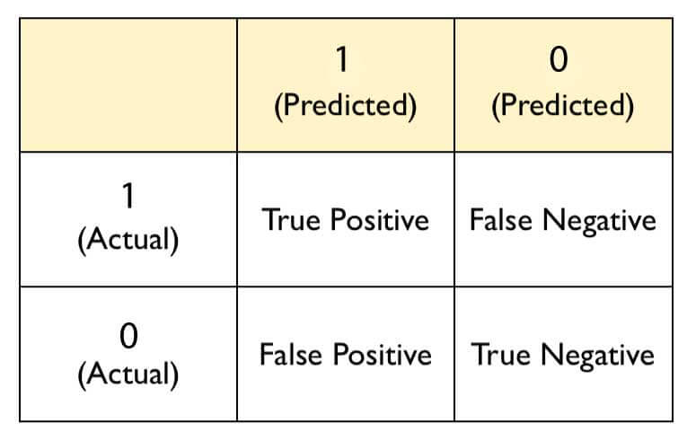
As you can see, the confusion matrix avoids "confusion" by measuring the actual and predicted values in a tabular format. In table above, Positive class = 1 and Negative class = 0. Following are the metrics we can derive from a confusion matrix:
Accuracy - It determines the overall predicted accuracy of the model. It is calculated as Accuracy = (True Positives + True Negatives)/(True Positives + True Negatives + False Positives + False Negatives)
True Positive Rate (TPR) - It indicates how many positive values, out of all the positive values, have been correctly predicted. The formula to calculate the true positive rate is (TP/TP + FN). Also, TPR = 1 - False Negative Rate. It is also known as Sensitivity or Recall.
False Positive Rate (FPR) - It indicates how many negative values, out of all the negative values, have been incorrectly predicted. The formula to calculate the false positive rate is (FP/FP + TN). Also, FPR = 1 - True Negative Rate.
True Negative Rate (TNR) - It indicates how many negative values, out of all the negative values, have been correctly predicted. The formula to calculate the true negative rate is (TN/TN + FP). It is also known as Specificity.
False Negative Rate (FNR) - It indicates how many positive values, out of all the positive values, have been incorrectly predicted. The formula to calculate false negative rate is (FN/FN + TP).
Precision: It indicates how many values, out of all the predicted positive values, are actually positive. It is formulated as:(TP / TP + FP). F Score: F score is the harmonic mean of precision and recall. It lies between 0 and 1. Higher the value, better the model. It is formulated as 2((precision*recall) / (precision+recall)).
4. Receiver Operator Characteristic (ROC)
ROC determines the accuracy of a classification model at a user defined threshold value. It determines the model's accuracy using Area Under Curve (AUC). The area under the curve (AUC), also referred to as index of accuracy (A) or concordant index, represents the performance of the ROC curve. Higher the area, better the model. ROC is plotted between True Positive Rate (Y axis) and False Positive Rate (X Axis). In this plot, our aim is to push the red curve (shown below) toward 1 (left corner) and maximize the area under curve. Higher the curve, better the model. The yellow line represents the ROC curve at 0.5 threshold. At this point, sensitivity = specificity.
Practical - Who survived the Titanic disaster?
For illustration, we'll be working on one of the most popular data sets in machine learning: Titanic. It's fairly small in size and a variety of variables will give us enough space for creative feature engineering and model building. This data set has been taken from Kaggle. I hope you know that model building is the last stage in machine learning. Therefore, we'll be doing quick data exploration, pre-processing, and feature engineering before implementing Logistic Regression. For your convenience, the data can downloaded from here.
#set working directory
> path <- "~Manish/Data/Titanic"
> setwd(path)

#load libraries and data
> library (data.table)
> library (plyr)
> library (stringr)
> train <- fread("train.csv",na.strings = c(""," ",NA,"NA"))
> test <- fread("test.csv",na.strings = c(""," ",NA,"NA"))
> head(train)
> head(test)
> str(train)
Survived is the dependent variable. To get a deeper understanding of these variables, let's do a quick data exploration. Discoveries from this step will help us determine what to do next:
#check missing values
> colSums(is.na(train))
> colSums(is.na(test))
Age and Cabin have missing values. Interestingly, the variable Fare has one missing value only in the test set. Let's start exploring each variable individually. For numeric variables, we'll use the summary function. For character / factor variables, we'll use table for exploration:
#Quick Data Exploration
> summary(train$Age)
> summary(test$Age)

> train[,.N/nrow(train),Pclass]
> test[,.N/nrow(test),Pclass]

> train [,.N/nrow(train),Sex]
> test [,.N/nrow(test),Sex]

> train [,.N/nrow(train),SibSp]
> test [,.N/nrow(test),SibSp]

> train [,.N/nrow(train),Parch]
> test [,.N/nrow(test),Parch] #extra 9

> summary(train$Fare)
> summary(test$Fare)

> train [,.N/nrow(train),Cabin]
> test [,.N/nrow(test),Cabin]

> train [,.N/nrow(train),Embarked]
> test [,.N/nrow(test),Embarked]
- The variable
Fareis skewed (right) in nature. We'll have to log transform it such that it resembles a normal distribution. - The variable
Parchhas one extra level (9) in the test set as compared to the train set. We'll have to combine it with its mode value.
A smart way to make modifications in train and test data is by combining them. This way, you'll save yourself from writing some extra lines of code. I suggest you follow every line of code carefully and simultaneously check how every line affects the data.
#combine data
> alldata <- rbind(train,test,fill=TRUE)
For now, we'll create two new variables. First, title of the passengers. This information can be extracted from Name. Second, I suspect that Ticket notation could give us some information. For example, some ticket notation starts with alpha numeric, while others only have numbers. We'll capture this trend using a binary coded variable.
#New Variables
#Extract passengers title
> alldata [,title := strsplit(Name,split = "[,.]")]
> alldata [,title := ldply(.data = title,.fun = function(x) x[2])]
> alldata [,title := str_trim(title,side = "left")]

#combine titles
> alldata [,title := replace(title, which(title %in% c("Capt","Col","Don","Jonkheer","Major","Rev","Sir")), "Mr"),by=title]
> alldata [,title := replace(title, which(title %in% c("Lady","Mlle","Mme","Ms","the Countess","Dr","Dona")),"Mrs"),by=title]

#ticket binary coding
> alldata [,abs_col := strsplit(x = Ticket,split = " ")]
> alldata [,abs_col := ldply(.data = abs_col,.fun = function(x)length(x))]
> alldata [,abs_col := ifelse(abs_col > 1,1,0)]
Fare variable and remove an extra level from Parch variable. This will make our data ready for machine learning.
#Impute Age with Median
> for(i in "Age")
        set(alldata,i = which(is.na(alldata[[i]])),j=i,value = median(alldata$Age,na.rm = T))

#Remove rows containing NA from Embarked
> alldata <- alldata[!is.na(Embarked)]

#Impute Fare with Median
> for(i in "Fare")
      set(alldata,i = which(is.na(alldata[[i]])),j=i,value = median(alldata$Fare,na.rm = T))

#Replace missing values in Cabin with "Miss"
> alldata [is.na(Cabin),Cabin := "Miss"]

#Log Transform Fare
> alldata$Fare <- log(alldata$Fare + 1)

#Impute Parch 9 to 0
> alldata [Parch == 9L, Parch := 0]
#Collect train and test
> train <- alldata[!(is.na(Survived))]
> train [,Survived := as.factor(Survived)]

> test <- alldata[is.na(Survived)]
> test [,Survived := NULL]

#Logistic Regression
> model <- glm(Survived ~ ., family = binomial(link = 'logit'), data = train[,-c("PassengerId","Name","Ticket")])
> summary(model)
glm function. Now, let's understand and interpret the crucial aspects of summary:
- The glm function internally encodes categorical variables into n - 1 distinct levels.
- Estimate represents the regression coefficients value. Here, the regression coefficients explain the change in log(odds) of the response variable for one unit change in the predictor variable.
- Std. Error represents the standard error associated with the regression coefficients.
- z value is analogous to t-statistics in multiple regression output. z value > 2 implies the corresponding variable is significant.
- p value determines the probability of significance of predictor variables. With 95% confidence level, a variable having p < 0.05 is considered an important predictor. The same can be inferred by observing stars against p value.
In addition, we can also perform an ANOVA Chi-square test to check the overall effect of variables on the dependent variable.
#run anova
> anova(model, test = 'Chisq')
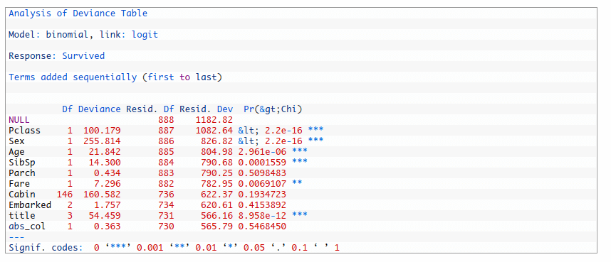
Following are the insights we can collect for the output above:
- In the presence of other variables, variables such as Parch, Cabin, Embarked, and abs_col are not significant. We'll try building another model without including them.
- The AIC value of this model is 883.79.
Let's create another model and try to achieve a lower AIC value.
> model2 <- glm(Survived ~ Pclass + Sex + Age + SibSp + Fare + title, data = train,family = binomial(link="logit"))
> summary(model2)
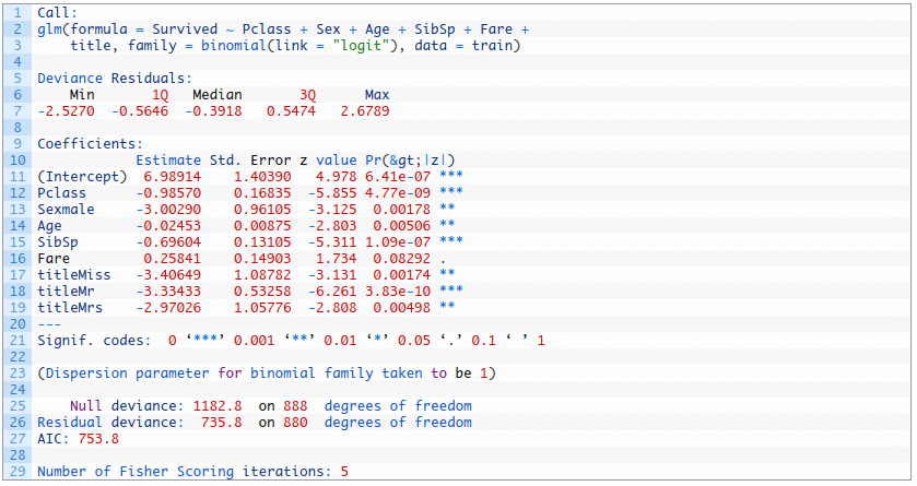
As you can see, we've achieved a lower AIC value and a better model. Also, we can compare both the models using the ANOVA test. Let's say our null hypothesis is that second model is better than the first model. p < 0.05 would reject our hypothesis and in case p > 0.05, we'll fail to reject the null hypothesis.
#compare two models
> anova(model,model2,test = "Chisq")
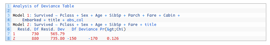
With p > 0.05, this ANOVA test also corroborates the fact that the second model is better than first model. Let's predict on unseen data now. Since, we can't evaluate a model's performance on test data locally, we'll divide the train set and use model 2 for prediction.
#partition and create training, testing data
> library(caret)
> split <- createDataPartition(y = train$Survived,p = 0.6,list = FALSE)

> new_train <- train[split]
> new_test <- train[-split]

#model training and prediction
> log_model <- glm(Survived ~ Pclass + Sex + Age + SibSp + Fare + title, data = new_train[,-c("PassengerId","Name","Ticket")],family = binomial(link="logit"))
> log_predict <- predict(log_model,newdata = new_test,type = "response")
> log_predict <- ifelse(log_predict > 0.5,1,0)
confusionMatrix function from caret package.
#plot ROC
> library(ROCR)
> library(Metrics)
> pr <- prediction(log_predict,new_test$Survived)
> perf <- performance(pr,measure = "tpr",x.measure = "fpr")
> plot(perf) > auc(new_test$Survived,log_predict) #0.76343
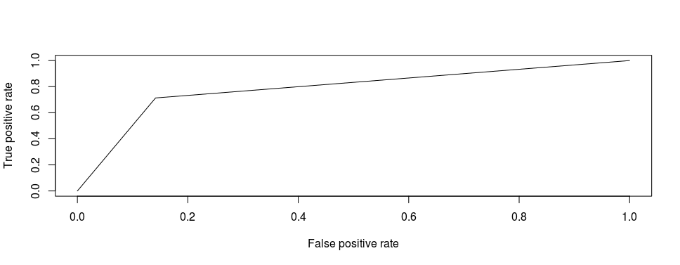
Our AUC score is 0.763. As said above, in ROC plot, we always try to move up and top left corner. From this plot, we can interpret that the model is predicting more negative values incorrectly. To move up, let's increase our threshold value to 0.6 and check the model's performance.
> log_predict <- predict(log_model,newdata = new_test,type = "response")
> log_predict <- ifelse(log_predict > 0.6,1,0)

> pr <- prediction(log_predict,new_test$Survived)
> perf <- performance(pr,measure = "tpr",x.measure = "fpr")
> plot(perf)
> auc(new_test$Survived,log_predict)` ` #0.8008
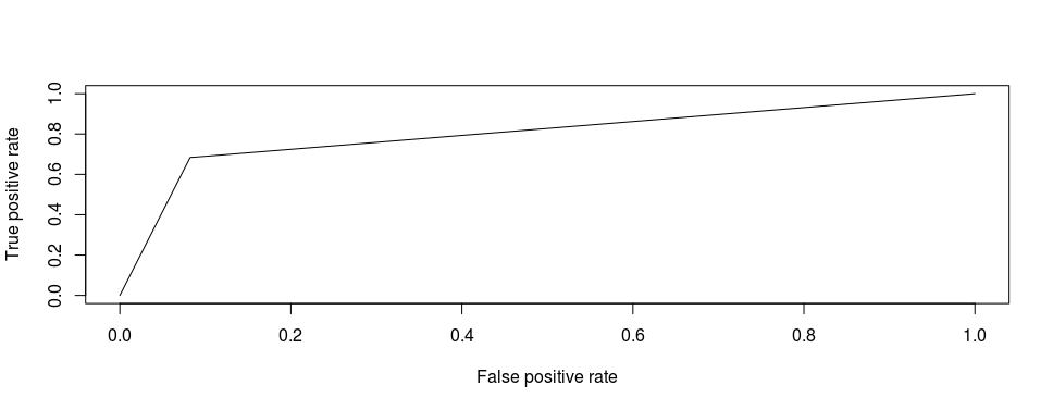
Now, our AUC has increased to 0.80 along with a slight uplift in the ROC curve. With this, we've reached to the end of this tutorial. You can try and test AUC value for other values of probability threshold as well. From here, I would request you go ahead and test your model on the original test set, upload your solution and check your kaggle rank. Moving beyond Logistic Regression, you can further improve your model's accuracy using tree-based algorithms such as Random Forest or XGBoost. The complete code for this tutorial is also available on Github.
Summary
This tutorial is meant to help people understand and implement Logistic Regression in R. Understanding Logistic Regression has its own challenges. No doubt, it is similar to Multiple Regression but differs in the way a response variable is predicted or evaluated. This tutorial is more than just machine learning. In the practical section, we also became familiar with important steps of data cleaning, pre-processing, imputation, and feature engineering.
While working on any classification problem, I would advise you to build your first model as Logistic Regression. The reason being that you might score a surprising accuracy even better than non-linear methods. If it's otherwise, you'd learn that the given data set would be better handled with non-linear methods, and you can use Logistic Regression's accuracy as your benchmark score.
While reading and practicing this tutorial, if there is anything you don't understand, don't hesitate to drop in your comments below!