
Deep Learning Challenge 2
Introduction
Deep Learning Challenge #2 was held from Dec 13, 2017, to Jan 31, 2018. More than 5000 participants took part in the competition but only a few persistently fought till the end. And those who didn’t give up and improved their model continuously by training and re-tuning ended up winning the challenge. The dataset in the problem was very large—with training data consisting of 18,577 images (approx. 7GB ) and testing dataset consisting of 12,836 images (5 GB). Such a large dataset did cause some difficulty for a few participants.
In this post, we’ll explore and analyse the dataset, create a model from scratch, and then look at the approaches adopted by the winners of this challenge.
Problem Statement
Chest X-ray exam is one of the most frequent and cost-effective medical imaging examinations. However, clinical diagnosis of a chest X-ray can be challenging, and, sometimes, believed to be harder than diagnosis via chest CT imaging. To achieve clinically relevant computer-aided detection and diagnosis (CAD) in real-world medical sites on all data settings of chest X-rays is still very difficult unless several thousands of images are employed for study.
As part of a research study to explore deep learning techniques, National Institute of Health Clinical Center (NIH) has recently open-sourced its dataset of frontal chest X-ray images of patients. The task was to identify the class of thorax diseases from the given chest x-ray images.
Data Exploration
We were given two separate datasets, one containing images and the other containing CSV files. The train data has information for 18,577 patients and test data has information for 12,386 patients. The target variable has 14 types of thorax diseases. Some part of the data was anonymised to restrict fraudulent submissions.
| Variable | Description |
|---|---|
| row_id | Unique patient id |
| age | Patient age |
| gender | Patient gender |
| view position | Position of Image (binary) |
| Image_name | X-ray image corresponding to patient |
| detected | Target variable |
Table 1. Description of data in the csv files.
#We import the required libraries for data exploration and visualization.

import pandas as pd
import matplotlib.pyplot as plt
import os
import numpy as np
import seaborn as sns
%matplotlib inline
The DL#2 consists of three CSV files (train, test and sample_submission) and two folders which consists of the train and the test images. The train and the test CSV files consist of the meta-data related to each patient’s X-ray images stored in the train and test image folders, respectively. Table 2 shows the metadata stored in train.csv for the first five patients.
#Next we read the datasets.

train = pd.read_csv('train.csv')
test = pd.read_csv('test.csv')
train.head()
| row_id | age | gender | view_position | Image_name | detected | |
|---|---|---|---|---|---|---|
| 0 | id_0 | 45 | M | 0 | scan_0000.png | class_3 |
| 1 | id_1 | 57 | F | 0 | scan_0001.png | class_3 |
| 2 | id_10 | 58 | M | 0 | scan_00010.png | class_3 |
| 3 | id_1000 | 64 | M | 0 | scan_0001000.png | class_6 |
| 4 | id_10000 | 33 | M | 1 | scan_00010000.png | class_3 |
Table 2. Information of the first five patients stored in train.csv
The target variable or the detected variable (as seen in Table 2) has 14 unique classes, each denoting a class of thorax disease.
Exploratory Visualization
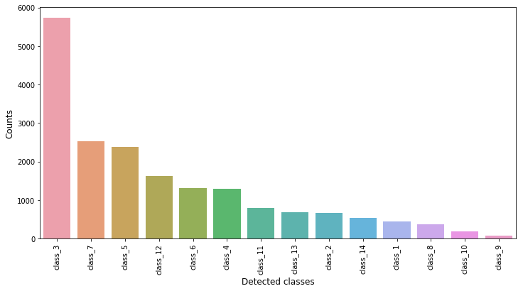
We now explore our dataset with the help of visual graphs and plots to get a better understanding of it. We use seaborn and matplotlib libraries to produce our visualisations. Fig 1. shows the occurrence/ frequency of each class in the target variable of the training dataset, sorted in the descending order. From the figure we can see that class_3 type thorax disease is more prominent in patients, while class_9 type thorax disease is quite rare.
#Distribution of the target variable.

detected_counts = train.detected.value_counts()
plt.figure(figsize = (12,6))
sns.barplot(detected_counts.index, detected_counts.values, alpha = 0.9)
plt.xticks(rotation = 'vertical')
plt.xlabel('Detected classes', fontsize =12)
plt.ylabel('Counts', fontsize = 12)
plt.show()
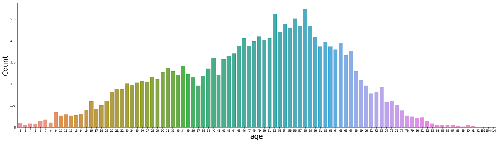
Next, we analyse the distribution of the variable ‘age’ in the training dataset. From Fig 2. we see that the ‘age’ of the patients is normally distributed. Also, it contains outliers, e.g. some patients in the training dataset have age in the range of 150–500 years, which seems to be incorrect and may misguide our training model.
#Distribution of the variable 'age'.

ax = plt.figure(figsize=(30, 8))
sns.countplot(train.age)
axis_font = {'fontname':'Arial', 'size':'24'}
plt.xlabel('age',  **axis_font)
plt.ylabel('Count',  **axis_font)
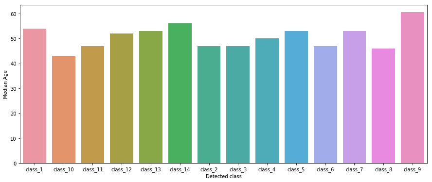
Fig. 3 shows the median age of patients for each type of class in the ‘detected’ (target) variable. We can see that class_9 type thorax disease is common in patients over the age of 60. We calculate the median of the variable ‘age’ for each target class, instead of the mean because of outliers in the data.
#Distribution of the variable 'age' over the target variable.

temp = train.groupby(['detected']).median()
ax = plt.figure(figsize=(15, 6))
sns.barplot(temp.index, temp.age)
plt.xlabel('Detected class')
plt.ylabel('Median Age')
Finally, we use the OpenCV(cv2) library for image manipulation. Other libraries such as PILLOW, PIL, or skimage can also be used. Unlike humans, a computer cannot recognise an image as it is. The computer cannot see shapes or colors. To a computer, any image is read as an array of numbers.
#Load the image data and visualise it USING Open CV.

TRAIN_PATH = 'train_/'
TEST_PATH = 'test_/'

import cv2
img = cv2.imread(TRAIN + 'scan_0000.png')
print(img.shape)
plt.imshow(img)
Each image in the training dataset is of the shape (1024, 1024, 3), where the first two numbers represent the number of rows of pixels and the number of columns of pixels. Number 3 represents the RGB color spectrum. Each number in the array represents a single pixel.
Data Preprocessing
Since each image in our dataset is an array of size 1024*1024*3, processing 18,577 images of size 1024*1024*3 requires enormous computation power. Therefore, we resize them to more appropriate sizes. Here, we resize each image in our dataset to 128*128*3 dimensions.
#We create a function, which reads an image, resizes it to 128 x128 dimensions and returns it.

def read_img(img_path):
    img = cv2.imread(img_path)
    img = cv2.resize(img, (128, 128))
    return img

from tqdm import tqdm
train_img = []
for img_path in tqdm(train['image_name'].values):
    train_img.append(read_img(TRAIN_PATH + img_path))
Next, we rescale our image data. Rescale is a value by which we will multiply the data before any other preprocessing. Our original images are made of RGB coefficients lying in the range 0–255, but such values will be too high for our models to process (given a typical learning rate), so we target values between 0 and 1 instead by scaling with a 1/255 factor.
#Rescaling the images

x_train = np.array(train_img, np.float32) / 255.
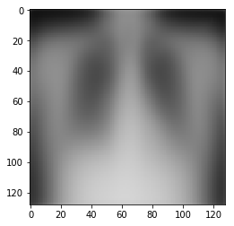
Next, we calculate the mean of all the training images. It is a good average representation of the entire training dataset. The mean image is calculated by taking the mean values for each pixel across all training examples. The image roughly represents the thorax (see Fig 4.) . This image lets us conclude that all the thoraxes are somewhat aligned to the center and are of comparable sizes.
#Mean of the images

mean_img = np.mean(x_train, axis=0)
plt.imshow(mean_img)

Following this, we calculate the standard deviation of the all images. High variance shows up whiter (see Fig. 5), so we can see that the pictures vary a lot at the lungs compared to the rest of the image.
#Standard deviation of the images

std_img = np.std(x_train, axis=0)
plt.imshow(std_img)
The reason we calculate the mean and standard deviation of the images is that in the process of training our network, we are going to be multiplying (weights) and adding (biases) to these initial inputs to cause activations, which get back-propagated with the gradients to train the model. We will like each feature to have a similar range so that our gradients don’t go out of control (and we only need one global learning rate multiplier).
Thus, we normalize both our train and test datasets. This is done using the following formula:
$x = Input array$
$μ = Mean value$
$σ = Standard deviation$
$X = Output/Resultant array$
#Normalization

x_train_norm = (x_train - mean_img) / std_img
x_train_norm.shape
Finally, we encode our target variables as the model needs an array of numbers to train. But for categorical variables where no ordinal relationship exists, integer encoding is not enough. In fact, using this encoding and allowing the model to assume a natural ordering between categories may result in poor performance or unexpected results. Therefore, we apply one-hot encoding to the integer representation of the categories. Here, the integer encoded variable is removed and a new binary variable is added for each unique integer value, for example, a one-hot encoded representation of the target variable can be:
Class_1 : 10000000000000
Class_2 : 01000000000000
Class_3 : 00100000000000, and so on.
#Encoding the target variable as integers

class_list = train['detected'].tolist()
Y_train = {k:v+1 for v,k in enumerate(set(class_list))}
y_train = [Y_train[k] for k in class_list]
#One-hot encoding the target variable.

from keras.utils import to_categorical
y_train = to_categorical(y_train)
Modelling
The most important part of a deep learning problem is to choose the appropriate training model. While choosing a model, we have two options: - Transfer learning: Where you transfer a pre-trained model and weights and fit it to your model - Create your own model: Here you create your own model from scratch and train its weights; this gives you better control over your model
We use the Keras framework to build our model. Keras is a high-level API written in Python. It runs on top Tensorflow, CNTK, or Theano. It is relatively easy to use and understand and is very fast.
#Importing the required libraries

from keras.models import Sequential
from keras.layers import Dense, Dropout, Flatten, Convolution2D, MaxPooling2D
from keras.callbacks import EarlyStopping
We create a Sequential model to solve this problem. A Deep learning model consists of a number of layers connects to each other. The input data is passed through each layer, one-by-one. We use a Sequential model which is a linear stack of layers.
#We create a Sequential model using 'categorical cross-entropy' as our loss function and 'adam' as the optimizer.

model = Sequential()
model.add(Convolution2D(32, (3,3), activation='relu', padding='same',input_shape = (128,128,3)))
#if you resize the image above, change the input shape
model.add(Convolution2D(32, (3,3), activation='relu'))
model.add(MaxPooling2D(pool_size=(2,2)))

model.add(Convolution2D(64, (3,3), activation='relu', padding='same'))
model.add(Convolution2D(64, (3,3), activation='relu'))
model.add(MaxPooling2D(pool_size=(2,2)))
model.add(Dropout(0.25))

model.add(Convolution2D(128, (3,3), activation='relu', padding='same'))
model.add(Convolution2D(128, (3,3), activation='relu'))
model.add(MaxPooling2D(pool_size=(2,2)))
model.add(Dropout(0.25))

model.add(Flatten())
model.add(Dense(128, activation='relu'))
model.add(Dense(256, activation='relu'))
model.add(Dropout(0.25))
model.add(Dense(y_train.shape[1], activation='softmax'))
model.compile(loss = 'categorical_crossentropy', optimizer = 'adam', metrics = ['accuracy'])
model.summary()
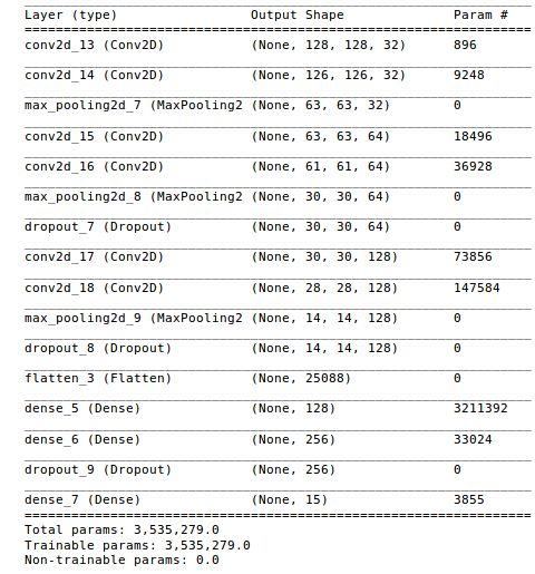
Fig. 6, gives a summary of our model architecture. The input shape (128*128) is passed at the very top of the model. This input is run through all the layers sequentially. We can see from the figure that our model has approximately 3.5 million parameters (weights) to train. We use ‘categorical cross entropy’ as the loss function and ‘adam’ as the optimizer.
#We define an early stopping condition for the model. If the val_acc is the same three times, the model stops.

early_stops = EarlyStopping(patience=3, monitor='val_acc')
We now train this model using the input data. An epoch is when the model runs through the entire data once. batch_size refers to the number of training examples utilised in one iteration. validation_split splits our data into 70% training and 30% validation. The following code splits the input data into batches of 100 images and runs them through the model 10 times.
#Training the model for 10 epochs.

model.fit(x_train_norm, y_train, batch_size=100, epochs=10, validation_split=0.3, callbacks=[early_stops])
Lastly, we use our trained model to predict the labels on the test dataset.
#Now that we have built and trained our model, it is time to predict the test data.

test_img = []
for img in tqdm(test['image_name'].values):
    test_img.append(read_img(TEST_PATH + img))

#Applying the same data-preprocessing steps on the test data.
x_test = np.array(test_img, np.float32) / 255.
x_test_norm = (test_img, np.float32) / 255.

#The test data is normalised

predictions = model.predict(x_test_norm)
predictions = np.argmax(predictions, axis= 1)

y_maps = dict()
y_maps = {v:k for k, v in Y_train.items()}
pred_labels = [y_maps[k] for k in predictions]

#Creating the submission file.
sub = pd.DataFrame({'row_id':test.row_id, 'detected':pred_labels})
sub.to_csv('submission.csv', index=False)
The submission produces a score of 0.267 on the public leaderboard. This model can be further improved.
Winner Approaches
Krzysztof Broncel, Rank 1st
Krzysztof Broncel, the winner of this competition, was kind enough to share his approach with us that got him the first rank on the public leaderboard. The main idea behind his solution was the use of transfer learning to improve the whole training process. He used the VGG16 model with the imagenet weights to implement transfer learning.
By visualizing the output label distribution, he found out the presence of unbalanced classes (as seen in Fig. 1) and found that the training the model with such an unbalanced class would be hard. To overcome this unbalance, he did some remarkable feature engineering. He decided to generate more images for classes where the number of examples was lower than a given threshold. To do this, he created a script that slightly modifies the original image and saves it into an output folder. As a result of this, he was able to create a training dataset with each target class having at least 1500 images. He also resized the original images in the training dataset to 512 * 512 dimensions. Apart from this, he also found a few cases in the training dataset where the age of the patients was greater than 100 (see Fig. 2). He decided to drop these examples from the training dataset.
Finally, to build a model in a really fast and robust way, he decided to use Keras and its built-in VGG16 model with imagenet weights. Since, training such a model on an average CPU can be hard and time consuming due to lack of physical memory and weak GPU, he decided to invest in AWS GPU instance (p2.xlarge). His final model consisted of a VGG16 network connected with two MLP layers (512 and 15 nodes). He trained the model for 100 epochs with a batch size of 32 images.
Here are some suggestions from Krzysztof for a participant to focus on while solving a challenge: - Maintain your work logs: The most important thing during the whole competition is to maintain a file with all input parameters and the corresponding output values. Thanks to this, he was able to modify his approach tens of times and still be able to see what he had already tried and why it didn’t work. Such a work log can drastically improve the overall performance. - Get more data: If possible, try to get or even generate more data to have balanced distribution of classes. - Size of the image: Having big images increases the neural network complexity, but we don’t want to lose important details. - Pay attention to the relation between your image size and model performance. Choose the optimum. - Computational power: Use GPU when working on CNNs. It drastically reduces the overall training time. - Outliers: When working with images eliminate outliers whenever possible.
Tomasz Banaś, Rank 2nd
Tomasz Banaś came second in this challenge and although according to him it was his first online challenge, he gave an outstanding performance. He said that in machine learning the most import thing is to search all data which you can use to train the model. So, apart from the image dataset provided for this challenge, he also used an external dataset (link to the external dataset) of lung X-ray images. Besides this, he also generated 10K images for classes which had small number of images. This helped in eliminating the class imbalance present in the target label.
In case of feature engineering, he generated new images with different sizes, random horizontal/ vertical shifts, random rotations and stored images in grayscale instead of RGB. The best combination that worked for him was having images with size in the range of 250 - 350 px, random horizontal/vertical shifts (0.1 of total width/ height), rotating images upto 10 degrees, and storing images in grayscale instead of RGB.
He decided to use transfer learning and tested a few network architectures: VGG16, VGG19, ResNet50. The best results he achieved was with ResNet50 with the original images resized to 350 x 350. He finally added a few dense layers to his model and final model for which he achieved the best result has the following architecture:
Flatten()
Dense(2048, activation='relu')
Dropout(0.5)
Dense(512, activation='relu')
Dropout(0.5)
Dense(NUM_CLASSES, activation='softmax')
Initially, he imported the ResNet50 architecture with imagenet weights (using the Keras library) and froze all the layers except the fully connected layer. He trained the model for 20 epochs using the Adam optimizer (with learning rate: 0.0001 and decay: 0.00001). Then he unfroze the last 35 layers and again trained the model for 20 epochs using the Adam optimizer (with learning rate: 0.0001, decay: 0.00000001). He used AWS (p2.xlarge) to train his model.(Source Code)
According to him, the five things a participant must focus on while solving such problems are: - Check how you can use existing pretrained models for your problem. - Search more data which you can use to train your model. Having more data is sometimes far more important than having a perfect model. - Create a log/ Excel file to keep track of all the models, parameters, and the associated results. - Always use a GPU, instead of a CPU, as it will save a lot of time while running your model. Make use of cheap GPU services from AWS/ Azure/ Google cloud and others. - Create a basic model which works and then add more advance techniques/ data/ feature engineering. It’s better to have a basic model which works than a very advance model which doesn’t.
Akhil Punia, Rank 3rd
Akhil Punia came in third in this challenge. His submission to the challenge was inspired by the ChexNet model, which is a 121-layer CNN that inputs a chest X-ray image and outputs the probability of pneumonia along with a heatmap localizing the areas of the most indicative of pneumonia (link). The ChexNet model was trained on a similar dataset of chest X-rays as provided by the NIH. Akhil used the same approach, as provided in the ChexNet model, to build his own model for this challenge.
Akhil’s model made use of Densely Connected Convolutional Network (DenseNet), which connects each layer to every other layer in a feed-forward fashion.Traditional CNNs with L layers have L connections, one between each layer and its subsequent layers, whereas DenseNet have L(L+1)/2 direct connections. Counter-intuitive effect of this dense connectivity pattern is that it requires fewer parameters than traditional convolutional networks as there is no need to relearn redundant feature maps.
Akhil’s final model is similar to the ChexNet model, except that Chexnet used 121-layered DenseNet, while his model used 169 layered DenseNet (DenseNet - 169). He used transfer learning and imported the DenseNet 169 architecture along with the pretrained weights using the Torch library. Akhil used the Pytorch framework to create his model. He did some data augmentation by flipping the images along the y-axis and resized the original images to 256 x 256 dimensions. Finally, he trained the model for 100 epochs with a batch size of 16 images per batch. He used cloud-based GPU (AWS/ Google cloud/ Floydhub, etc.) to train his model.(Source Code)
Here are some suggestions from Akhil for a participant to focus on while solving such problems: - Look for similar problem statements and what standard procedures have been implemented to solve them. - Look for cheap cloud-based GPU (AWS/ Google cloud/ Floydhub) for training your model. - Instead of working on the whole dataset, work on a sample of the whole dataset to check if your model is behaving predictably.
Conclusion
Before we end the blog, let’s quickly summarize what we have learned. - Data Analysis and Exploration: Data analysis and exploration is a crucial step for understanding any dataset. As seen, it was because of this step that we were able to detect the unbalance present in the target labels. Also, we were able to find the presence of outliers in the dataset (using the ‘age’ distribution). All winners of this challenge used some kind of data analysis to observe this. - Outliers: Always try to eliminate or drop any outliers present in the dataset. - Get more data: If possible, try to get, or even generate, more data to have balanced distribution of classes. All winner approaches talk about this and consider it an important step in training the model. - Instead of building the model from scratch, check how you can use an existing pretrained model for your problem. All the winners used some kind of transfer learning to create their model as this could be more efficient. - Size of the image: Using big images increases the neural network complexity, hence we should always try to use images with low dimensions, without losing important details. - Maintain a log file: Every winner approach talks of maintaining some kind of log/ excel file of the models, parameters, and the corresponding result as it can help in improving the performance of the model. - Use of GPU: Try to use a GPU instead of a CPU as it will save a lot of time. One can use cheap cloud-based GPUs.
If this article makes you want to learn more about this dataset, I suggest you read this paper by Xiaosong Wang. Have anything to say? Feel free to drop your suggestions, recommendations, or concerns in comments below.