
Introduction
The ability to deal with text data is one of the important skills a data scientist must posses. With advent of social media, forums, review sites, web page crawlers companies now have access to massive behavioural data of their customers.
Yes, companies have more of textual data than numerical data. No doubt, this data will be messy. But, beneath it lives an enriching source of information, insights which can help companies to boost their businesses. That is the reason, why natural language processing (NLP) a.k.a Text Mining as a technique is growing rapidly and being extensively used by data scientists.
In the previous tutorial, we learnt about regular expressions in detail. Make sure you've read it.
In this tutorial, you'll about text mining from scratch. We'll follow a stepwise pedagogy to understand text mining concepts. Later, we'll work on a current kaggle competition data sets to gain practical experience, which is followed by two practice exercises. For this tutorial, the programming language used is R. However, the techniques explained below can be implemented in any programming language.
Table of Contents
- What is Text Mining (or Natural Language Processing ) ?
- What are the steps involved in Text Mining ?
- What are the feature engineering techniques used in Text Mining ?
- Text Mining Practical - Predict the interest level
What is Text Mining (or Natural Language Processing) ?
Natural Language Processing (NLP) or Text mining helps computers to understand human language. It involves a set of techniques which automates text processing to derive useful insights from unstructured data. These techniques helps to transform messy text data sets into a structured form which can be used into machine learning.
The resultant structured data sets are high dimensional i.e. large rows and columns. In a way, text expands the universe of data manifolds. Hence, to avoid long training time, you should be careful in choosing the ML algorithm for text data analysis. Generally, algorithms such as naive bayes, glmnet, deep learning tend to work well on text data.
What are the steps involved in Text Mining ?
Let's say you are given a data set having product descriptions. And, you are asked to extract features from the given descriptions. How would you start to make sense out of it ? The raw text data (description) will be filtered through several cleaning phases to get transformed into a tabular format for analysis. Let's look at some of the steps:
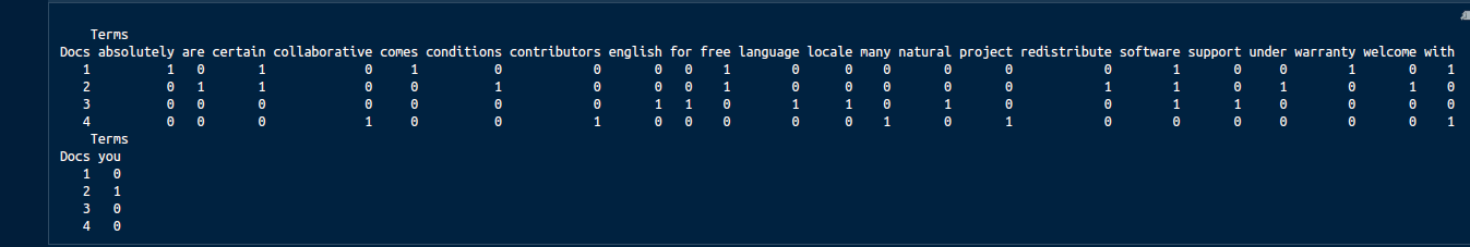
- Corpus Creation - It involves creating a matrix comprising of documents and terms (or tokens). A document can be understood as each row having product description and each column having terms. Terms refers to each word in the description. Usually, the number of documents in the corpus equals to number of rows in the given data.
Let's say our document is "Free software comes with ABSOLUTELY NO certain WARRANTY","You are welcome to redistribute free software under certain conditions","Natural language support for software in an English locale","A collaborative project with many contributors". The image below shows the matrix format of this document where every column represents a term from the document.
- Text Cleaning - It involves cleaning the text in following ways:
- Remove words - If the data is extracted using web scraping, you might want to remove html tags.
- Remove stop words - Stop words are a set of words which helps in sentence construction and don't have any real information. Words such as a, an, the, they, where etc. are categorized as stop words.
- Convert to lower - To maintain a standarization across all text and get rid of case differences and convert the entire text to lower.
- Remove punctuation - We remove punctuation since they don't deliver any information.
- Remove number - Similarly, we remove numerical figures from text
- Remove whitespaces - Then, we remove the used spaces in the text.
- Stemming & Lemmatization - Finally, we convert the terms into their root form. For example: Words like playing, played, plays gets converted to the root word 'play'. It helps in capturing the intent of terms precisely.
- Feature Engineering - To be explained in the following section
- Model Building - After the raw data is passed through all the above steps, it become ready for model building. As mentioned above, not all ML algorithms perform well on text data. Naive Bayes is popularly known to deliver high accuracy on text data. In addition, deep neural network models also perform fairly well.
What are Feature Engineering Techniques used in Text Mining ?
Do you know each word of this line you are reading can be converted into a feature ? Yes, you heard correctly. Text data offers a wide range of possibilities to generate new features. But sometimes, we end up generating lots of features, to an extent that processing them becomes a painful task. Hence we should meticulously analyze the extracted features. Don't worry! The methods explained below will also help in reducing the dimension of the resultant data set.
Below is the list of popular feature engineering methods used:
1. n-grams : In the document corpus, 1 word (such as baby, play, drink) is known as 1-gram. Similarly, we can have 2-gram (baby toy, play station, diamond ring), 3-gram etc. The idea behind this technique is to explore the chances that when one or two or more words occurs together gives more information to the model.
2. TF - IDF : It is also known as Term Frequency - Inverse Document Frequency. This technique believes that, from a document corpus, a learning algorithm gets more information from the rarely occurring terms than frequently occurring terms. Using a weighted scheme, this technique helps to score the importance of terms. The terms occurring frequently are weighted lower and the terms occurring rarely get weighted higher. * TF is be calculated as: frequency of a term in a document / all the terms in the document. * IDF is calculated as: ratio of log (total documents in the corpus / number of documents with the 'term' in the corpus) * Finally, TF-IDF is calculated as: TF X IDF. Fortunately, R has packages which can do these calculations effort
3. Cosine Similarity - This measure helps to find similar documents. It's one of the commonly used distance metric used in text analysis. For a given 2 vectors A and B of length n each, cosine similarity can be calculated as a dot product of two unit vectors:

4. Jaccard Similarity - This is another distance metric used in text analysis. For a given two vectors (A and B), it can be calculated as ratio of (terms which are available in both vectors / terms which are available in either of the vectors). It's formula is: (A ∩ B)/(A U B). To create features using distance metrics, first we'll create cluster of similar documents and assign a unique label to each document in a new column.
5. Levenshtein Distance - We can also use levenshtein distance to create a new feature based on distance between two strings. We won't go into its complicated formula, but understand what it does: it finds the shorter string in longer texts and returns the maximum value as 1 if both the shorter string is found. For example: Calculating levenshtein distance for string "Alps Street 41" and "1st Block, Alps Street 41" will result in 1.
6. Feature Hashing - This technique implements the 'hashing trick' which helps in reducing the dimension of document matrix (lesser columns). It doesn't use the actual data, instead it uses the indexes[i,j] of the data, thus it processes data only when needed. And, that's why it takes lesser memory in computation. In addition, there are more techniques which we'll discover while modeling text data in the next section.
Text Mining Practical - Predict the interest level
You can't become better at machine learning just by reading, coding is an inevitable aspect of it. Now, let's code and build some text mining models in R.
In this section, we'll try to incorporate all the steps and feature engineering techniques explained above. Since regular expressions help wonderfully in dealing with text data, make sure that you have referred to the regular expression tutorial as well. Instead of a dummy data, we'll get our hands on a real text mining problem. In this problem, we'll predict the popularity of apartment rental listing based on given features.
The data set has been taken from currently running two sigma rental listing problem on Kaggle. Therefore, after you finish this tutorial, you can right away participate in it and try your luck. Since the focus of this tutorial is text mining, we'll work only on the text features available in the data. For this tutorial, you can download the data here.
Now, we'll load the data and useful libraries for solving this problem. Using map_at function from purrr package, we'll convert the json files into tabular data tables.
#load libraries
path <- "/home/manish/Desktop/Data2017/February/twosigma/"
setwd(path)
library(data.table)
library(jsonlite)
library(purrr)
library(RecordLinkage)
library(stringr)
library(tm)

#load data
traind <- fromJSON("train.json")
test <- fromJSON("test.json")

#convert json to data table
vars <- setdiff(names(traind),c("photos","features"))
train <- map_at(traind, vars, unlist) %>% as.data.table()
test <- map_at(test,vars,unlist) %>% as.data.table()
Since we are interested only in text variables, let's extract the text features:
train <- train[,.(listing_id,features, description,street_address,display_address,interest_level)]
test <- test[,.(listing_id,features,street_address,display_address,description)]
Let's quickly understand what the data is about:
dim(train)
dim(test)
head(train)
head(test)
sapply(train,class)
sapply(test,class)
From the analysis above, we can derive the following insights:
- The train data has 49352 rows and 6 columns. The test data has 74659 rows and 5 columns.
- interest_level is the dependent variable i.e. the variable to predict
- listing_id variable has unique value for every listing. In other words, it is the identifier variable.
- features comprises of a list of features for every listing_id
- description refers to the description of a listing_id provided by the agent
- Street address and display address refers to the address of the listed apartment.
Let's start with the analysis.
We'll now join the data and create some new features.
#join data
test[,interest_level := "None"]
tdata <- rbindlist(list(train,test))

#fill empty values in the list
tdata[,features := ifelse(map(features, is_empty),"aempty",features)]

#count number of features per listing
tdata[,feature_count := unlist(lapply(features, length))]

#count number of words in description
tdata[,desc_word_count := str_count(description,pattern = "\\w+")]

#count total length of description
tdata[,desc_len := str_count(description)]

#similarity between address
tdata[,lev_sim := levenshteinDist(street_address,display_address)]
Feature engineering doesn't play by a fixed set of rules. With a different data set, you'll always discover new potential set of features. The best way to become at expert at feature engineering is solve different types of problems. Anyhow, for this problem I've created the following variables:
- Count of number of features per listing
- Count of number of words in the description
- Count of total length of the description
- Similarity between street and display address using levenshtein distance
dim(tdata)
Now, the data has 10 variables and 680961 observations. If you think these variables are too less for a machine learning algorithm to work best, hold tight. In a while, our data dimension is going to explode. We'll create more new features from the variable 'Features' and 'Description'.
Let's take them up one by one. First, we'll transform the list 'Features' into one feature per row format.
#extract variables from features
fdata <- data.table(listing_id = rep(unlist(tdata$listing_id), lapply(tdata$features, length)), features = unlist(tdata$features))
head(fdata)

#convert features to lower
fdata[,features := unlist(lapply(features, tolower))]
Since not all the features will be useful, let's calculate the count of features and remove features which are occurring less than 100 times in the data.
#calculate count for every feature
fdata[,count := .N, features]
fdata[order(count)][1:20]

#keep features which occur 100 or more times
fdata <- fdata[count >= 100]
Let's convert each feature into a separate column so that it can be used as a variable in model training. To accomplish that, we'll use the dcast function.
#convert columns into table`<br/>
fdata <- dcast(data = fdata, formula = listing_id ~ features, fun.aggregate = length, value.var = "features")
dim(fdata)
This has resulted in 96 new variables. We'll keep this new data set as is, and extract more features from the description variable. From here, we'll be using tm package.
#create a corpus of descriptions
text_corpus <- Corpus(VectorSource(tdata$description))
#check first 4 documents
inspect(text_corpus[1:4])

#the corpus is a list object in R of type CORPUS
print(lapply(text_corpus[1:2], as.character))
As you can see, the word 'br' is just a noise and doesn't provide any useful information in the description. We'll remove it. Also, we'll perform the text mining steps to clean the data as explained in section above.
#let's clean the data
dropword <- "br"

#remove br
text_corpus <- tm_map(text_corpus,removeWords,dropword)
print(as.character(text_corpus[[1]]))

#tolower
text_corpus <- tm_map(text_corpus, tolower)
print(as.character(text_corpus[[1]]))

#remove punctuation
text_corpus <- tm_map(text_corpus, removePunctuation)
print(as.character(text_corpus[[1]]))

#remove number
text_corpus <- tm_map(text_corpus, removeNumbers)
print(as.character(text_corpus[[1]]))

#remove whitespaces
text_corpus <- tm_map(text_corpus, stripWhitespace,lazy = T)
print(as.character(text_corpus[[1]]))

#remove stopwords
text_corpus <- tm_map(text_corpus, removeWords, c(stopwords('english')))
print(as.character(text_corpus[[1]]))

#convert to text document
text_corpus <- tm_map(text_corpus, PlainTextDocument)

#perform stemming - this should always be performed after text doc conversion
text_corpus <- tm_map(text_corpus, stemDocument,language = "english")
print(as.character(text_corpus[[1]]))
text_corpus[[1]]$content
After every cleaning step, we've printed the resultant corpus to help you understand the effect of each step on the corpus. Now, our corpus is ready to get converted into a matrix.
#convert to document term matrix
docterm_corpus <- DocumentTermMatrix(text_corpus)
dim(docterm_corpus)
Let's remove the variables which are 95% or more sparse.
new_docterm_corpus <- removeSparseTerms(docterm_corpus,sparse = 0.95)
dim(new_docterm_corpus)
#find frequent terms
colS <- colSums(as.matrix(new_docterm_corpus))
length(colS)
doc_features <- data.table(name = attributes(colS)$names, count = colS)
#most frequent and least frequent words
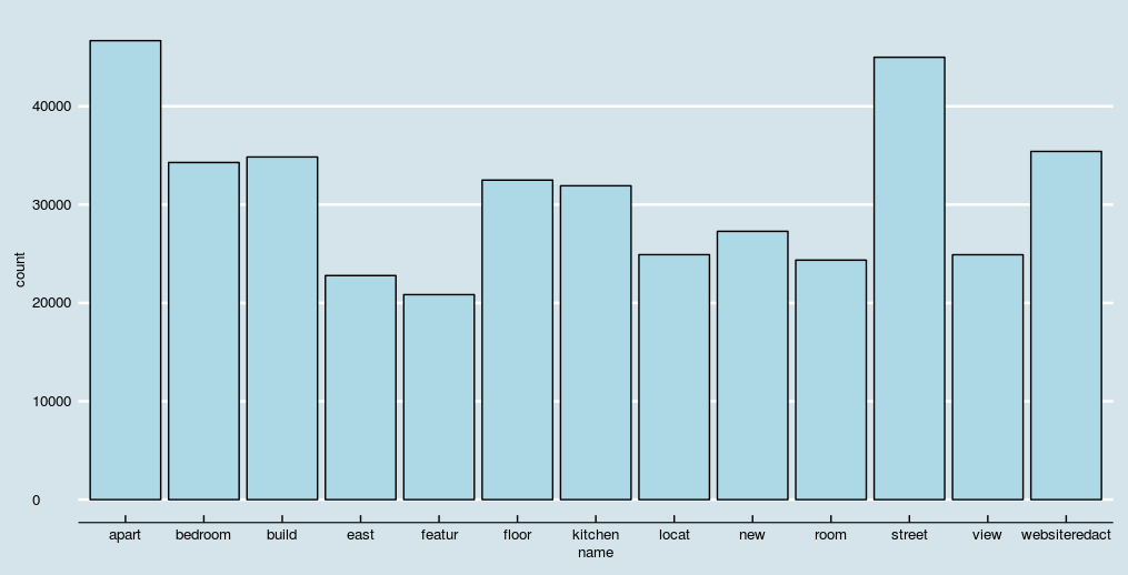
doc_features[order(-count)][1:10] #top 10 most frequent words
doc_features[order(count)][1:10] #least 10 frequent words
library(ggplot2)
library(ggthemes)

ggplot(doc_features[count>20000],aes(name, count)) +` `geom_bar(stat = "identity",fill='lightblue',color='black')+` `theme(axis.text.x = element_text(angle = 45, hjust = 1))+` `theme_economist()+` `scale_color_economist()` <br/>
#check association of terms of top features
findAssocs(new_docterm_corpus,"street",corlimit = 0.5)
findAssocs(new_docterm_corpus,"new",corlimit = 0.5)
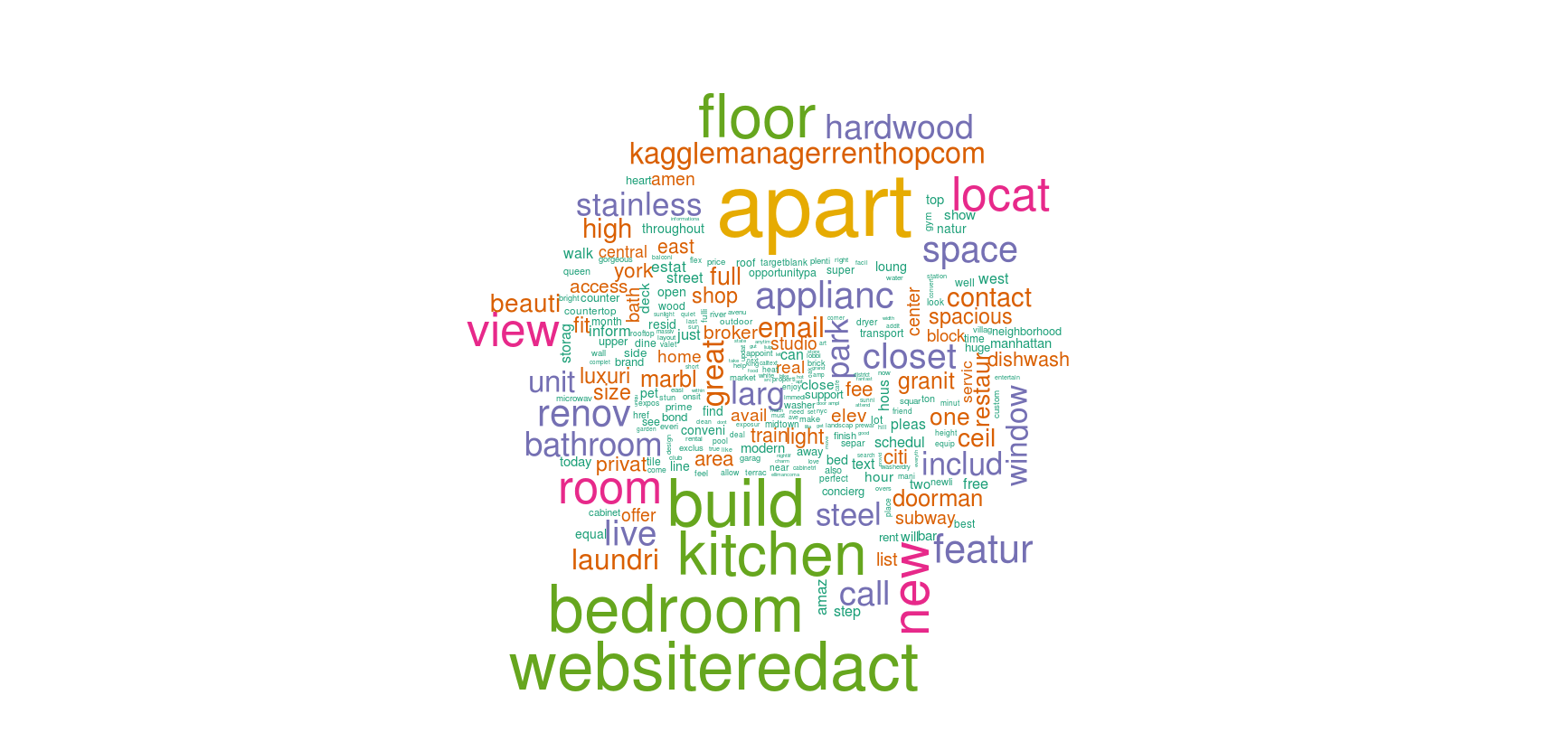
#create wordcloud
library(wordcloud)
wordcloud(names(colS), colS, min.freq = 100, scale = c(6,.1), colors = brewer.pal(6, 'Dark2'))
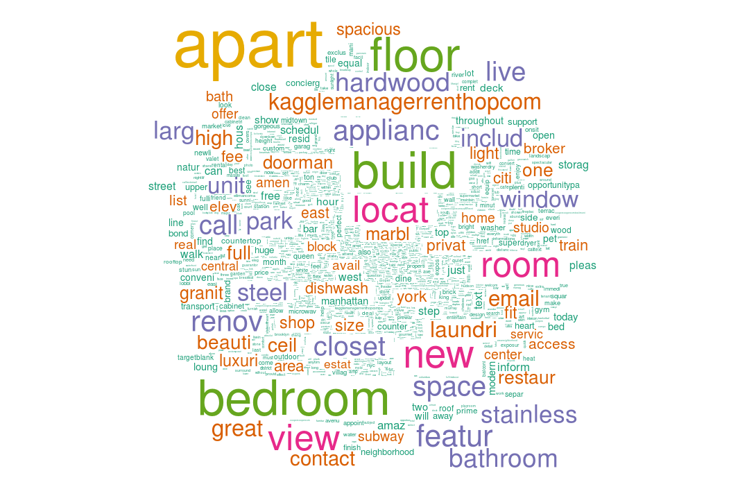
wordcloud(names(colS), colS, min.freq = 5000, scale = c(6,.1), colors = brewer.pal(6, 'Dark2'))
Until here, we've chopped the description variable and extracted 87 features out of it. The final step is to convert the matrix into a data frame and merge it with new features from 'Feature' column.
#create data set for training
processed_data <- as.data.table(as.matrix(new_docterm_corpus))

#combing the data
data_one <- cbind(data.table(listing_id = tdata$listing_id, interest_level = tdata$interest_level),processed_data)

#merging the features
data_one <- fdata[data_one, on="listing_id"]

#split the data set into train and test
train_one <- data_one[interest_level != "None"]
test_one <- data_one[interest_level == "None"]
test_one[,interest_level := NULL]
Xgboost follows a certain way of dealing with data:
- It accepts dependent variable in integer format.
- The data should be in matrix format
- To check model performance, we can specify a validation set such that we can check validation errors during model training. It is enable with both k-fold and hold-out validation strategy. For faster training, we'll use hold-out validation strategy.
- The training data must not have dependent variable. It should be removed. Neither, it should have the identifier variable (listing_id)
Keeping its nature in mind, let's prepare the data for xgboost and train our model.
library(caTools)
library(xgboost)

#stratified splitting the data
sp <- sample.split(Y = train_one$interest_level,SplitRatio = 0.6)

#create data for xgboost
xg_val <- train_one[sp]
listing_id <- train_one$listing_id
target <- train_one$interest_level

xg_val_target <- target[sp]

d_train <- xgb.DMatrix(data = as.matrix(train_one[,-c("listing_id","interest_level"),with=F]),label = target)
d_val <- xgb.DMatrix(data = as.matrix(xg_val[,-c("listing_id","interest_level"),with=F]), label = xg_val_target)
d_test <- xgb.DMatrix(data = as.matrix(test_one[,-c("listing_id"),with=F]))

param <- list(booster="gbtree", objective="multi:softprob", eval_metric="mlogloss",  num_class=3, eta = .02, gamma = 1, max_depth = 4, min_child_weight = 1, subsample = 0.7, colsample_bytree = 0.5)

set.seed(2017)
watch <- list(val=d_val, train=d_train)

xgb2 <- xgb.train(data = d_train, params = param, watchlist=watch, nrounds = 500, print_every_n = 10)
This model returns validation error = 0.6817. The score is calculated with multilogloss metric. Think of validation error as a proxy performance of model on future data. Now, let's create predictions on test data and check our score on kaggle leaderboard.
xg_pred <- as.data.table(t(matrix(predict(xgb2, d_test), nrow=3, ncol=nrow(d_test))))
colnames(xg_pred) <- c("high","low","medium")

xg_pred <- cbind(data.table(listing_id = test$listing_id),xg_pred)
fwrite(xg_pred, "xgb_textmining.csv")
What about TF-IDF matrix ? Here's an exercise for you. We created processed_data as a data table from new_docterm_corpus. It contained simple 1 and 0 to detect the presence of a new word in the description. Let's create a weighted matrix using tf-idf technique. It's quite easy to do.
#TF IDF Data set
data_mining_tf <- as.data.table(as.matrix(weightTfIdf(new_docterm_corpus)))
Does your score improve ? What else can be done ? Think! What about n - gram technique ? Until now, our matrix has one gram features i.e. one word per column such as apart, new, building etc. Now, we'll create a 2-gram document matrix and check model performance on it. To create a n-gram matrix, we'll use NGramTokenizer function from Rweka package.
install.packages("RWeka")
library(RWeka)

#bigram function
Bigram_Tokenizer <- function(x){` `NGramTokenizer(x, Weka_control(min=2, max=2))` `}

#create a matrix
bi_docterm_matrix <- DocumentTermMatrix(text_corpus, control = list(tokenize = Bigram_Tokenizer))
bi_docterm_matrix and check your score. Your next steps would are similar to what we've done above. For your reference, following are the steps you should take:
- Remove sparse terms
- Explore the new features using bar chart and wordcloud
- Convert the matrix into data table
- Divide the resultant data table into train and test
- Train and Test the models
Once this is done, check the leaderboard score. Do let me know in comments if it got improved. The complete script of this tutorial can be found here.
Summary
This tutorial is meant for beginners to get started with building text mining models. Considering the massive volume of content being generated by companies, social media these days, there is going to be a surge in demand for people who are well versed with text mining & natural language processing.
This tutorial illustrates all the necessary steps which one must take while dealing with text data. For better understanding, I would suggest you to get your hands on variety of text data sets and use the steps above for analysis. Regardless of any programming language you use, these techniques & steps are common in all. Did you find this tutorial helpful ? Feel free to drop your suggestions, doubts in the comments below.