
Graph traversals
Graph traversal means visiting every vertex and edge exactly once in a well-defined order. While using certain graph algorithms, you must ensure that each vertex of the graph is visited exactly once. The order in which the vertices are visited are important and may depend upon the algorithm or question that you are solving.
During a traversal, it is important that you track which vertices have been visited. The most common way of tracking vertices is to mark them.
Breadth First Search (BFS)
There are many ways to traverse graphs. BFS is the most commonly used approach.
BFS is a traversing algorithm where you should start traversing from a selected node (source or starting node) and traverse the graph layerwise thus exploring the neighbour nodes (nodes which are directly connected to source node). You must then move towards the next-level neighbour nodes.
As the name BFS suggests, you are required to traverse the graph breadthwise as follows:
- First move horizontally and visit all the nodes of the current layer
- Move to the next layer
Consider the following diagram.
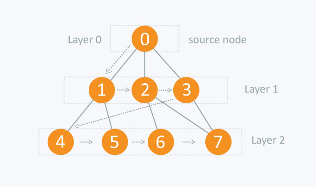
The distance between the nodes in layer 1 is comparitively lesser than the distance between the nodes in layer 2. Therefore, in BFS, you must traverse all the nodes in layer 1 before you move to the nodes in layer 2.
Traversing child nodes
A graph can contain cycles, which may bring you to the same node again while traversing the graph. To avoid processing of same node again, use a boolean array which marks the node after it is processed. While visiting the nodes in the layer of a graph, store them in a manner such that you can traverse the corresponding child nodes in a similar order.
In the earlier diagram, start traversing from 0 and visit its child nodes 1, 2, and 3. Store them in the order in which they are visited. This will allow you to visit the child nodes of 1 first (i.e. 4 and 5), then of 2 (i.e. 6 and 7), and then of 3 (i.e. 7) etc.
To make this process easy, use a queue to store the node and mark it as 'visited' until all its neighbours (vertices that are directly connected to it) are marked. The queue follows the First In First Out (FIFO) queuing method, and therefore, the neigbors of the node will be visited in the order in which they were inserted in the node i.e. the node that was inserted first will be visited first, and so on.
Pseudocode
BFS (G, s)                   //Where G is the graph and s is the source node
      let Q be queue.
      Q.enqueue( s ) //Inserting s in queue until all its neighbour vertices are marked.

      mark s as visited.
      while ( Q is not empty)
           //Removing that vertex from queue,whose neighbour will be visited now
           v  =  Q.dequeue( )

          //processing all the neighbours of v
          for all neighbours w of v in Graph G
               if w is not visited
                        Q.enqueue( w )             //Stores w in Q to further visit its neighbour
                        mark w as visited.
Traversing process
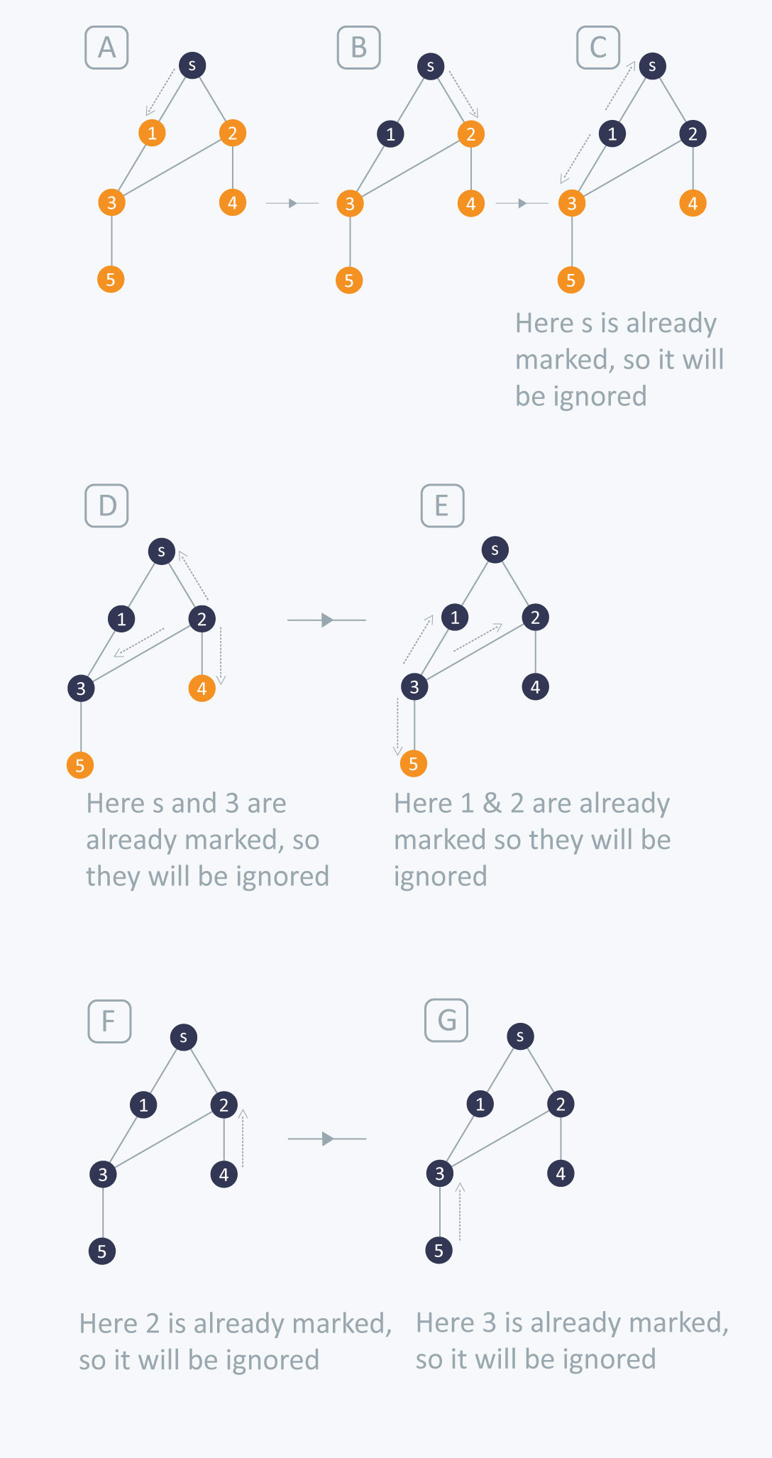
The traversing will start from the source node and push s in queue. s will be marked as 'visited'.
First iteration
- s will be popped from the queue
- Neighbors of s i.e. 1 and 2 will be traversed
- 1 and 2, which have not been traversed earlier, are traversed. They will be:
- Pushed in the queue
- 1 and 2 will be marked as visited
Second iteration
- 1 is popped from the queue
- Neighbors of 1 i.e. s and 3 are traversed
- s is ignored because it is marked as 'visited'
- 3, which has not been traversed earlier, is traversed. It is:
- Pushed in the queue
- Marked as visited
Third iteration
- 2 is popped from the queue
- Neighbors of 2 i.e. s, 3, and 4 are traversed
- 3 and s are ignored because they are marked as 'visited'
- 4, which has not been traversed earlier, is traversed. It is:
- Pushed in the queue
- Marked as visited
Fourth iteration
- 3 is popped from the queue
- Neighbors of 3 i.e. 1, 2, and 5 are traversed
- 1 and 2 are ignored because they are marked as 'visited'
- 5, which has not been traversed earlier, is traversed. It is:
- Pushed in the queue
- Marked as visited
Fifth iteration
- 4 will be popped from the queue
- Neighbors of 4 i.e. 2 is traversed
- 2 is ignored because it is already marked as 'visited'
Sixth iteration
- 5 is popped from the queue
- Neighbors of 5 i.e. 3 is traversed
- 3 is ignored because it is already marked as 'visited'
The queue is empty and it comes out of the loop. All the nodes have been traversed by using BFS.
If all the edges in a graph are of the same weight, then BFS can also be used to find the minimum distance between the nodes in a graph.
Example
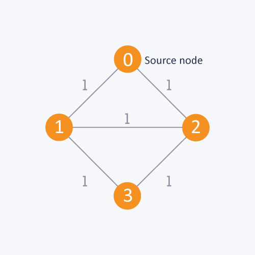
As in this diagram, start from the source node, to find the distance between the source node and node 1. If you do not follow the BFS algorithm, you can go from the source node to node 2 and then to node 1. This approach will calculate the distance between the source node and node 1 as 2, whereas, the minimum distance is actually 1. The minimum distance can be calculated correctly by using the BFS algorithm.
Complexity
The time complexity of BFS is O(V + E), where V is the number of nodes and E is the number of edges.
Applications
1. How to determine the level of each node in the given tree?
As you know in BFS, you traverse level wise. You can also use BFS to determine the level of each node.
Implementation
   vector <int> v[10] ;   //Vector for maintaining adjacency list explained above
    int level[10]; //To determine the level of each node
    bool vis[10]; //Mark the node if visited
    void bfs(int s) {
        queue <int> q;
        q.push(s);
        level[ s ] = 0 ;  //Setting the level of the source node as 0
        vis[ s ] = true;
        while(!q.empty())
        {
            int p = q.front();
            q.pop();
            for(int i = 0;i < v[ p ].size() ; i++)
            {
                if(vis[ v[ p ][ i ] ] == false)
                {
            //Setting the level of each node with an increment in the level of parent node
                    level[ v[ p ][ i ] ] = level[ p ]+1;
                     q.push(v[ p ][ i ]);
                     vis[ v[ p ][ i ] ] = true;
      }
            }
        }
    }
This code is similar to the BFS code with only the following difference:
level[ v[ p ][ i ] ] = level[ p ]+1;
In this code, while you visit each node, the level of that node is set with an increment in the level of its parent node. This is how the level of each node is determined.
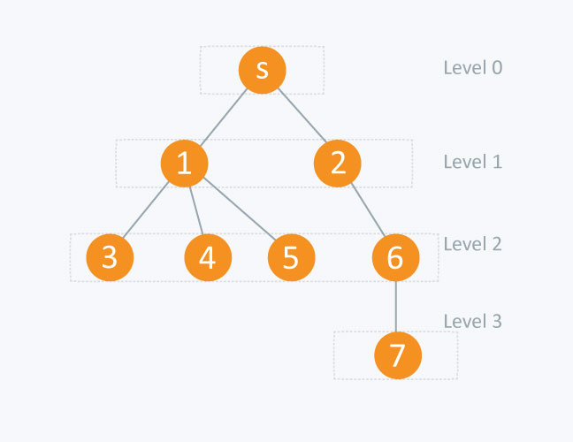
          node                            level [node]

              s (source node)               0
              1                            1
              2                            1
              3                            2
              4                            2
              5                            2
              6                            2
              7                            3
2. 0-1 BFS
This type of BFS is used to find the shortest distance between two nodes in a graph provided that the edges in the graph have the weights 0 or 1. If you apply the BFS explained earlier in this article, you will get an incorrect result for the optimal distance between 2 nodes.
In this approach, a boolean array is not used to mark the node because the condition of the optimal distance will be checked when you visit each node. A double-ended queue is used to store the node. In 0-1 BFS, if the weight of the edge = 0, then the node is pushed to the front of the dequeue. If the weight of the edge = 1, then the node is pushed to the back of the dequeue.
Implementation
Here, edges[ v ] [ i ] is an adjacency list that exists in the form of pairs i.e. edges[ v ][ i ].first will contain the node to which v is connected and edges[ v ][ i ].second will contain the distance between v and edges[ v ][ i ].first.
Q is a double-ended queue. The distance is an array where, distance[ v ] will contain the distance from the start node to v node. Initially the distance defined from the source node to each node is infinity.
void bfs (int start)
{
            deque <int > Q;     //Double-ended queue
            Q.push_back( start);
            distance[ start ] = 0;
            while( !Q.empty ())
            {
                int v = Q.front( );
                Q.pop_front();
                for( int i = 0 ; i < edges[v].size(); i++)
               {


/* if distance of neighbour of v from start node is greater than sum of distance of v from start node and edge weight between v and its neighbour (distance between v and its neighbour of v) ,then change it */


                    if(distance[ edges[ v ][ i ].first ] > distance[ v ] + edges[ v ][ i ].second )
                {

                    distance[ edges[ v ][ i ].first ] = distance[ v ] + edges[ v ][ i ].second;

                /*if edge weight between v and its neighbour is 0 then push it to front of
        double ended queue else push it to back*/

                    if(edges[ v ][ i ].second == 0)
                    {
                        Q.push_front( edges[ v ][ i ].first);
                    }
                    else
                    {
                            Q.push_back( edges[ v ][ i ].first);

                    }
                }
              }
           }
    }
Let’s understand this code with the following graph:
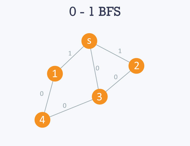
The adjacency list of the graph will be as follows:
Here 's' is considered to be 0 or source node.
0 -> 1 -> 3 -> 2
edges[ 0 ][ 0 ].first = 1 , edges[ 0 ][ 0 ].second = 1
edges[ 0 ][ 1 ].first = 3 , edges[ 0 ][ 1 ].second = 0
edges[ 0 ][ 2 ].first = 2 , edges[ 0 ][ 2 ].second = 1
1 -> 0 -> 4
edges[ 1 ][ 0 ].first = 0 , edges[ 1 ][ 0 ].second = 1
edges[ 1 ][ 1 ].first = 4 , edges[ 1 ][ 1 ].second = 0
2 -> 0 -> 3
edges[ 2 ][ 0 ].first = 0 , edges[ 2 ][ 0 ].second = 0
edges[ 2 ][ 1 ].first = 3 , edges[ 2 ][ 1 ].second = 0
3 -> 0 -> 2 -> 4
edges[ 3 ][ 0 ].first = 0 , edges[ 3 ][ 0 ].second = 0
edges[ 3 ][ 2 ].first = 2 , edges[ 3 ][ 2 ].second = 0
edges[ 3 ][ 3 ].first = 4 , edges[ 3 ][ 3 ].second = 0
4 -> 1 -> 3
edges[ 4 ][ 0 ].first = 1 , edges[ 4 ][ 0 ].second = 0
edges[ 4 ][ 1 ].first = 3 , edges[ 4 ][ 1 ].second = 0
If you use the BFS algorithm, the result will be incorrect because it will show you the optimal distance between s and node 1 and s and node 2 as 1 respectively. This is because it visits the children of s and calculates the distance between s and its children, which is 1. The actual optimal distance is 0 in both cases.
Processing
Starting from the source node, i.e 0, it will move towards 1, 2, and 3. Since the edge weight between 0 and 1 and 0 and 2 is 1 respectively, 1 and 2 will be pushed to the back of the queue. However, since the edge weight between 0 and 3 is 0, 3 will pushed to the front of the queue. The distance will be maintained in distance array accordingly.
3 will then be popped from the queue and the same process will be applied to its neighbours, and so on.