
Articulation Point
In a graph, a vertex is called an articulation point if removing it and all the edges associated with it results in the increase of the number of connected components in the graph. For example consider the graph given in following figure.
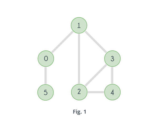
If in the above graph, vertex 1 and all the edges associated with it, i.e. the edges 1-0, 1-2 and 1-3 are removed, there will be no path to reach any of the vertices 2, 3 or 4 from the vertices 0 and 5, that means the graph will split into two separate components. One consisting of the vertices 0 and 5 and another one consisting of the vertices 2, 3 and 4 as shown in the following figure.
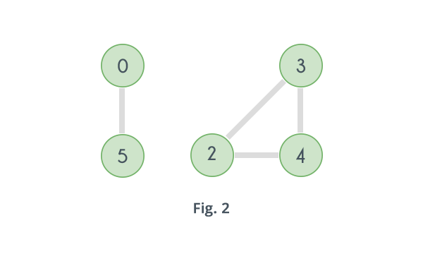
Likewise removing the vertex 0 will disconnect the vertex 5 from all other vertices. Hence the given graph has two articulation points: 0 and 1.
Articulation Points represents vulnerabilities in a network. In order to find all the articulation points in a given graph, the brute force approach is to check for every vertex if it is an articulation point or not, by removing it and then counting the number of connected components in the graph. If the number of components increases then the vertex under consideration is an articulation point otherwise not.
Here's the pseudo code of the brute force approach, it returns the total number of articulation points in the given graph.
function find_articulation_points(adj[][], V)
    count = 0
    for i = 0 to V
        visited[i] = false
    initial_val = 0
    for i = 0 to V
        if visited[i] == false
            DFS(adj, V, visited, i)
            initial_val = initial_val+1

    for i=0 to V
        for j = 0 to V
            visited[j] = false
            copy[j] = adj[i][j]
            adj[i][j]=adj[j][i]=0

        nval = 0
        for j= 0 to V
            if visited[j] == false AND j != i
                nval = nval + 1
                DFS(adj, n, visited, j)
        if nval > initial_val
            count = count + 1
        for j= 0 to V
            adj[i][j] = adj[j][i] = copy[j]
    return count
The above algorithm iterates over all the vertices and in one iteration applies a Depth First Search to find connected components, so time complexity of above algorithm is $$O(V \times (V+E))$$, where V is the number of vertices and E is the number of edges in the graph.
Clearly the brute force approach will fail for bigger graphs.
There is an algorithm that can help find all the articulation points in a given graph by a single Depth First Search, that means with complexity $$O(V+E)$$, but it involves a new term called "Back Edge" which is explained below:
Given a DFS tree of a graph, a Back Edge is an edge that connects a vertex to a vertex that is discovered before it's parent. For example consider the graph given in Fig. 1. The figure given below depicts a DFS tree of the graph.
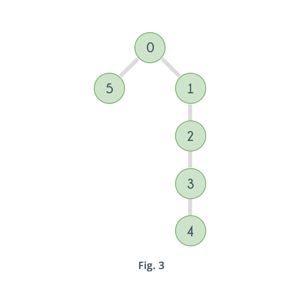
In the above case, the edge 4 - 2 connects 4 to an ancestor of its parent i.e. 3, so it is a Back Edge. And similarly 3 - 1 is also a Back edge. But why bother about Back Edge? Presence of a back edge means presence of an alternative path in case the parent of the vertex is removed. Suppose a vertex $$u$$ is having a child $$v$$ such that none of the vertices in the subtree rooted at $$v$$ have a back edge to any vertex discovered before $$u$$, that means if vertex $$u$$ is removed then there will be no path left for vertex $$v$$ or any of the vertices present in the subtree rooted at vertex v to reach any vertex discovered before $$u$$, that implies, the subtree rooted at vertex $$v$$ will get disconnected from the entire graph, and thus the number of components will increase and $$u$$ will be counted as an articulation point. On the other hand, if the subtree rooted at vertex $$v$$ has a vertex $$x$$ that has back edge that connects it to a vertex discovered before $$u$$, say $$y$$, then there will be a path for any vertex in subtree rooted at $$v$$ to reach $$y$$ even after removal of $$u$$, and if that is the case with all the children of $$u$$, then $$u$$ will not count as an articulation point.
So ultimately it all converges down to finding a back edge for every vertex. So, for that apply a DFS and record the discovery time of every vertex and maintain for every vertex $$v$$ the earliest discovered vertex that can be reached from any of the vertices in the subtree rooted at $$v$$. If a vertex $$u$$ is having a child $$v$$ such that the earliest discovered vertex that can be reached from the vertices in the subtree rooted at $$v$$ has a discovery time greater than or equal to $$u$$, then $$v$$ does not have a back edge, and thus $$u$$ will be an articulation point.
So, till now the algorithm says that if all children of a vertex $$u$$ are having a back edge, then $$u$$ is not an articulation point. But what will happen when $$u$$ is root of the tree, as root does not have any ancestors. Well, it is very easy to check if the root is an articulation point or not. If root has more than one child than it is an articulation point otherwise it is not. Now how does that help?? Suppose root has two children, $$v_1$$ and $$v_2$$. If there had been an edge between vertices in the subtree rooted at $$v_1$$ and those of the subtree rooted at $$v_2$$, then they would have been a part of the same subtree.
Here's the pseudo code of the above algorithm:
time = 0
function DFS(adj[][], disc[], low[], visited[], parent[], AP[], vertex, V)
        visited[vertex] = true
        disc[vertex] = low[vertex] = time+1
        child = 0
        for i = 0 to V
                if adj[vertex][i] == true
                        if visited[i] == false
                                child = child + 1
                                parent[i] = vertex
                                DFS(adj, disc, low, visited, parent, AP, i, n, time+1)
                                low[vertex] = minimum(low[vertex], low[i])
                                if parent[vertex] == nil and child > 1
                                        AP[vertex] = true
                                if parent[vertex] != nil and low[i] >= disc[vertex]
                                        AP[vertex] = true
                        else if parent[vertex] != i
                                low[vertex] = minimum(low[vertex], disc[i])
Here's what everything means:
$$adj[][]$$ : It is an $$N \times N$$ matrix denoting the adjacency matrix of the given graph.
$$disc[]$$ : It is an array of $$N$$ elements which stores the discovery time of every vertex. It is initialized by 0.
$$low[]$$ : It is an array of $$N$$ elements which stores, for every vertex $$v$$, the discovery time of the earliest
discovered vertex to which $$v$$ or any of the vertices in the subtree rooted at $$v$$ is having a back edge. It is initialized by INFINITY.
$$visited[]$$ : It is an array of size $$N$$ which denotes whether a vertex is visited or not during the DFS. It is initialized by false.
$$parent[]$$ : It is an array of size $$N$$ which stores the parent of each vertex. It is initialized by NIL.
$$AP[]$$ : It is an array of size $$N$$. $$AP[i]$$ = true, if ith vertex is an articulation point.
$$vertex$$: The vertex under consideration.
$$V$$ : Number of vertices.
$$time$$ : Current value of discovery time.
The above algorithm starts with an initial vertex say $$u$$, marks it visited, record its discovery time, $$disc[u]$$, and since it is just discovered, the earliest vertex it is connected to is itself, so $$low[u]$$ is also set equal to vertex's discovery time.
It keeps a counter called $$child$$ to count the number of children of a vertex. Then the algorithm iterates over every vertex in the graph and see if it is connected to $$u$$, if it finds a vertex $$v$$. that is connected to $$u$$, but has already been visited, then it updates the value $$low[u]$$ to minimum of $$low[u]$$ and discovery time of $$v$$ i.e., $$disc[v]$$.But if the vertex $$v$$ is not yet visited, then it sets the $$parent[v]$$ to $$u$$ and calls the DFS again with $$vertex = v$$. So the same things that just happened with $$u$$ will happen for $$v$$ also. When that DFS call will return, $$low[v]$$ will have the discovery time of the earliest discovered vertex that can be reached from any vertex in the subtree rooted at $$v$$. So set $$low[u]$$ to minimum of $$low[v]$$ and itself. And finally if $$u$$ is not the root, it checks whether $$low[v]$$ is greater than or equal to $$disc[u]$$, and if so, it marks $$AP[u]$$ as true. And if $$u$$ is root it checks whether it has more than one child or not, and if so, it marks $$AP[u]$$ as true.
The following image shows the value of array $$disc[]$$ and $$low[]$$ for DFS tree given in Fig. 3.
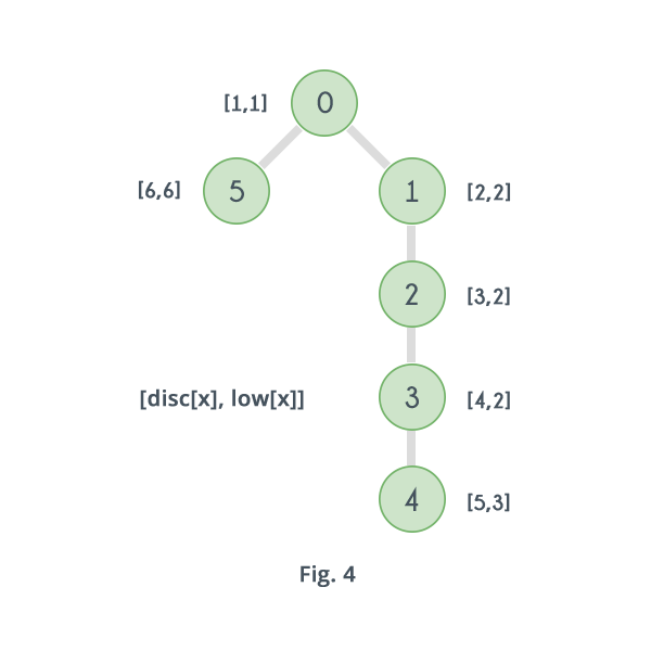
Clearly only for vertices 0 and 1, $$low[ 5 ] \ge disc[ 0 ]$$ and $$low[ 2 ] \ge disc[ 1 ]$$, so these are the only two articulation points in the given graph.
Bridges
An edge in a graph between vertices say $$u$$ and $$v$$ is called a Bridge, if after removing it, there will be no path left between $$u$$ and $$v$$. It's definition is very similar to that of Articulation Points. Just like them it also represents vulnerabilities in the given network. For the graph given in Fig.1, if the edge 0-1 is removed, there will be no path left to reach from 0 to 1, similarly if edge 0-5 is removed, there will be no path left that connects 0 and 5. So in this case the edges 0-1 and 0-5 are the Bridges in the given graph.
The Brute force approach to find all the bridges in a given graph is to check for every edge if it is a bridge or not, by first removing it and then checking if the vertices that it was connecting are still connected or not. Following is pseudo code of this approach:
function find_bridges(adj[][], V, Edge[], E, isBridge[])
    for i = 0 to E
        adj[Edge[i].u][Edge[i].v]=adj[Edge[i].v][Edge[i].u]=0
        for j = 0 to V
            visited[j] = false
        Queue.Insert(Edge[i].u])
        visited[Edge[i].u] = true
        check = false
        while Queue.isEmpty() == false
            x = Queue.top()
            if x == Edge[i].v
                check = true
                BREAK
            Queue.Delete()
            for j = 0 to V
                if adj[x][j] == true AND visited[j] == false
                    Queue.insert(j)
                    visited[j] = true
        adj[Edge[i].u][Edge[i].v]=adj[Edge[i].v][Edge[i].u]=1
        if check == false
            isBridge[i] = true
The above code uses BFS to check if the vertices that were connected by the removed edge are still connected or not. It does so for every edge and thus it's complexity is $$O(E \times (V+E))$$. Clearly it will fail for big values of $$V$$ and $$E$$.
To check if an edge is a bridge or not the above algorithm checks if the vertices that the edge is connecting are connected even after removal of the edge or not. If they are still connected, this implies existence of an alternate path. So just like in the case of Articulation Points the concept of Back Edge can be used to check the existence of the alternate path. For any edge, $$u - v$$, (u having discovery time less than v), if the earliest discovered vertex that can be visited from any vertex in the subtree rooted at vertex $$v$$ has discovery time strictly greater than that of $$u$$, then $$u - v$$ is a Bridge otherwise not. Unlike articulation point, here root is not a special case. Following is the pseudo code for the algorithm:
time = 0
function DFS(adj[][], disc[], low[], visited[], parent[], vertex, n)
        visited[vertex] = true
        disc[vertex] = low[vertex] = time+1
        child = 0
        for i = 0 to n
                if adj[vertex][i] == true
                        if visited[i] == false
                                child = child + 1
                                parent[i] = vertex
                                DFS(adj, disc, low, visited, parent, i, n, time+1)
                                low[vertex] = minimum(low[vertex], low[i])
                                if low[i] > disc[vertex]
                                        print vertex, i
                        else if parent[vertex] != i
                                low[vertex] = minimum(low[vertex], disc[i])
For graph given in Fig.1, the $$low[]$$ and $$disc[]$$ value obtained for its DFS tree shown in Fig.3, by the above pseudo code, will be the same as those obtained in case of articulation points. The values of array $$low[]$$ and $$disc[]$$ are shown in Fig.4. Clearly for only two edges i.e 0-1 and 0-5, $$low[ 1 ]$$ > $$ disc[0] $$ and $$ low[5] $$ > $$ disc[0] $$, hence those are the only two bridges in the given graph.